This Jupyter notebook can be downloaded from rednoise-fit-example.ipynb, or viewed as a python script at rednoise-fit-example.py.
Red noise and DM noise fitting examples
This notebook provides an example on how to fit for red noise and DM noise using PINT using simulated datasets.
We will use the PLRedNoise and PLDMNoise models to generate noise realizations (these models provide Fourier Gaussian process descriptions of achromatic red noise and DM noise respectively).
We will fit the generated datasets using the WaveX and DMWaveX models, which provide deterministic Fourier representations of achromatic red noise and DM noise respectively.
Finally, we will convert the WaveX/DMWaveX amplitudes into spectral parameters and compare them with the injected values.
[1]:
from pint import DMconst
from pint.models import get_model
from pint.simulation import make_fake_toas_uniform
from pint.logging import setup as setup_log
from pint.fitter import WLSFitter
from pint.utils import (
    dmwavex_setup,
    find_optimal_nharms,
    wavex_setup,
    plrednoise_from_wavex,
    pldmnoise_from_dmwavex,
)

from io import StringIO
import numpy as np
import astropy.units as u
from matplotlib import pyplot as plt
from copy import deepcopy

setup_log(level="WARNING")
[1]:
1
Red noise fitting
Simulation
The first step is to generate a simulated dataset for demonstration. Note that we are adding PHOFF as a free parameter. This is required for the fit to work properly.
[2]:
par_sim = """
    PSR           SIM3
    RAJ           05:00:00     1
    DECJ          15:00:00     1
    PEPOCH        55000
    F0            100          1
    F1            -1e-15       1
    PHOFF         0            1
    DM            15           1
    TNREDAMP      -13
    TNREDGAM      3.5
    TNREDC        30
    TZRMJD        55000
    TZRFRQ        1400
    TZRSITE       gbt
    UNITS         TDB
    EPHEM         DE440
    CLOCK         TT(BIPM2019)
"""

m = get_model(StringIO(par_sim))
[3]:
# Now generate the simulated TOAs.
ntoas = 2000
toaerrs = np.random.uniform(0.5, 2.0, ntoas) * u.us
freqs = np.linspace(500, 1500, 8) * u.MHz

t = make_fake_toas_uniform(
    startMJD=53001,
    endMJD=57001,
    ntoas=ntoas,
    model=m,
    freq=freqs,
    obs="gbt",
    error=toaerrs,
    add_noise=True,
    add_correlated_noise=True,
    name="fake",
    include_bipm=True,
    include_gps=True,
    multi_freqs_in_epoch=True,
)
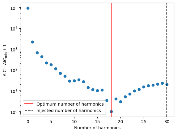
Optimal number of harmonics
The optimal number of harmonics can be estimated by minimizing the Akaike Information Criterion (AIC). This is implemented in the pint.utils.find_optimal_nharms function.
[4]:
m1 = deepcopy(m)
m1.remove_component("PLRedNoise")

nharm_opt, d_aics = find_optimal_nharms(m1, t, "WaveX", 30)

print("Optimum no of harmonics = ", nharm_opt)
Optimum no of harmonics = 15
[5]:
print(np.argmin(d_aics))
15
[6]:
# The Y axis is plotted in log scale only for better visibility.
plt.scatter(list(range(len(d_aics))), d_aics + 1)
plt.axvline(nharm_opt, color="red", label="Optimum number of harmonics")
plt.axvline(
    int(m.TNREDC.value), color="black", ls="--", label="Injected number of harmonics"
)
plt.xlabel("Number of harmonics")
plt.ylabel("AIC - AIC$_\\min{} + 1$")
plt.legend()
plt.yscale("log")
# plt.savefig("sim3-aic.pdf")
[7]:
# Now create a new model with the optimum number of harmonics
m2 = deepcopy(m1)
Tspan = t.get_mjds().max() - t.get_mjds().min()
wavex_setup(m2, T_span=Tspan, n_freqs=nharm_opt, freeze_params=False)

ftr = WLSFitter(t, m2)
ftr.fit_toas(maxiter=10)
m2 = ftr.model

print(m2)
# Created: 2024-05-02T16:05:31.075095
# PINT_version: 1.0+54.g0e607ed
# User: docs
# Host: build-24258979-project-85767-nanograv-pint
# OS: Linux-5.19.0-1028-aws-x86_64-with-glibc2.35
# Python: 3.11.6 (main, Feb  1 2024, 16:47:41) [GCC 11.4.0]
# Format: pint
PSR                                  SIM3
EPHEM                               DE440
CLOCK                        TT(BIPM2019)
UNITS                                 TDB
START              53000.9999999567007408
FINISH             56985.0000000464821181
DILATEFREQ                              N
DMDATA                                  N
NTOA                                 2000
CHI2                   1984.3477915130732
CHI2R                  1.0108750848258141
TRES                0.9920729073072599945
RAJ                      5:00:00.00016465 1 0.00009374255810320811
DECJ                    14:59:59.98018029 1 0.01086956282910487952
PMRA                                  0.0
PMDEC                                 0.0
PX                                    0.0
F0                  100.00000000000040225 1 4.4588321254685192691e-13
F1              -9.997288392948596479e-16 1 1.8054883758439291037e-19
PEPOCH             55000.0000000000000000
PLANET_SHAPIRO                          N
DM                 14.9999913842997639225 1 4.8266415168836399315e-06
WXEPOCH            55000.0000000000000000
WXFREQ_0001         0.0002510040160586007
WXSIN_0001         -5.439024192239741e-06 1 4.995057063379143e-07
WXCOS_0001         -1.796772940101199e-05 1 1.0905494259799844e-05
WXFREQ_0002         0.0005020080321172014
WXSIN_0002          8.256780834724877e-08 1 2.532985280450281e-07
WXCOS_0002         2.9927834111956714e-06 1 2.769130247390268e-06
WXFREQ_0003         0.0007530120481758023
WXSIN_0003         -1.235377849743115e-06 1 1.7585702104330788e-07
WXCOS_0003        -2.4739641154344977e-06 1 1.2664747315060804e-06
WXFREQ_0004         0.0010040160642344029
WXSIN_0004         -4.033703454601264e-07 1 1.3993427211435445e-07
WXCOS_0004          1.369635004940161e-06 1 7.446896974646336e-07
WXFREQ_0005         0.0012550200802930037
WXSIN_0005          5.962832090800399e-07 1 1.2197587497784874e-07
WXCOS_0005        -1.3335494252881996e-06 1 5.070611465130173e-07
WXFREQ_0006         0.0015060240963516046
WXSIN_0006         -2.246535583492585e-07 1 1.1247551589346571e-07
WXCOS_0006          6.811563095339189e-07 1 3.8590358396689103e-07
WXFREQ_0007         0.0017570281124102052
WXSIN_0007          8.273914038226498e-08 1 1.1204751192159644e-07
WXCOS_0007         -5.527642939098721e-07 1 3.2146842059727164e-07
WXFREQ_0008         0.0020080321284688058
WXSIN_0008         -6.509557726010107e-08 1 1.2008002972624713e-07
WXCOS_0008          3.703148530406356e-07 1 2.9765833025084734e-07
WXFREQ_0009          0.002259036144527407
WXSIN_0009         3.1294103519263826e-08 1 1.485185562444591e-07
WXCOS_0009         -6.481791483216267e-07 1 3.1849128689326337e-07
WXFREQ_0010         0.0025100401605860074
WXSIN_0010        -3.9659664380630315e-07 1 2.526657401875636e-07
WXCOS_0010           7.40973805471102e-07 1 4.774513807235659e-07
WXFREQ_0011          0.002761044176644608
WXSIN_0011        -1.9683952741710575e-06 1 2.043563952673017e-06
WXCOS_0011          5.993850506867757e-06 1 3.3766113292352807e-06
WXFREQ_0012          0.003012048192703209
WXSIN_0012         4.3212501994757195e-08 1 1.487697650599433e-07
WXCOS_0012           -3.5376790745702e-07 1 2.108490091665782e-07
WXFREQ_0013         0.0032630522087618097
WXSIN_0013        -1.2078026697892692e-07 1 7.080981378052525e-08
WXCOS_0013         1.0968973177218232e-07 1 8.673363787514832e-08
WXFREQ_0014         0.0035140562248204103
WXSIN_0014         1.0567904972761383e-07 1 4.8253848543838934e-08
WXCOS_0014         -1.169003640726403e-07 1 5.202010072404461e-08
WXFREQ_0015          0.003765060240879011
WXSIN_0015        -1.3504549682384328e-07 1 3.8933018828683806e-08
WXCOS_0015         1.6664885061599313e-07 1 3.963109745695271e-08
TZRMJD             55000.0000000000000000
TZRSITE                               gbt
TZRFRQ                             1400.0
PHOFF             -0.00036635413801635783 1 0.0009019379476080309
Estimating the spectral parameters from the WaveX fit.
[8]:
# Get the Fourier amplitudes and powers and their uncertainties.
idxs = np.array(m2.components["WaveX"].get_indices())
a = np.array([m2[f"WXSIN_{idx:04d}"].quantity.to_value("s") for idx in idxs])
da = np.array([m2[f"WXSIN_{idx:04d}"].uncertainty.to_value("s") for idx in idxs])
b = np.array([m2[f"WXCOS_{idx:04d}"].quantity.to_value("s") for idx in idxs])
db = np.array([m2[f"WXCOS_{idx:04d}"].uncertainty.to_value("s") for idx in idxs])
print(len(idxs))

P = (a**2 + b**2) / 2
dP = ((a * da) ** 2 + (b * db) ** 2) ** 0.5

f0 = (1 / Tspan).to_value(u.Hz)
fyr = (1 / u.year).to_value(u.Hz)
15
[9]:
# We can create a `PLRedNoise` model from the `WaveX` model.
# This will estimate the spectral parameters from the `WaveX`
# amplitudes.
m3 = plrednoise_from_wavex(m2)
print(m3)
# Created: 2024-05-02T16:05:31.119253
# PINT_version: 1.0+54.g0e607ed
# User: docs
# Host: build-24258979-project-85767-nanograv-pint
# OS: Linux-5.19.0-1028-aws-x86_64-with-glibc2.35
# Python: 3.11.6 (main, Feb  1 2024, 16:47:41) [GCC 11.4.0]
# Format: pint
PSR                                  SIM3
EPHEM                               DE440
CLOCK                        TT(BIPM2019)
UNITS                                 TDB
START              53000.9999999567007408
FINISH             56985.0000000464821181
DILATEFREQ                              N
DMDATA                                  N
NTOA                                 2000
CHI2                   1984.3477915130732
CHI2R                  1.0108750848258141
TRES                0.9920729073072599945
RAJ                      5:00:00.00016465 1 0.00009374255810320811
DECJ                    14:59:59.98018029 1 0.01086956282910487952
PMRA                                  0.0
PMDEC                                 0.0
PX                                    0.0
F0                  100.00000000000040225 1 4.4588321254685192691e-13
F1              -9.997288392948596479e-16 1 1.8054883758439291037e-19
PEPOCH             55000.0000000000000000
PLANET_SHAPIRO                          N
DM                 14.9999913842997639225 1 4.8266415168836399315e-06
TZRMJD             55000.0000000000000000
TZRSITE                               gbt
TZRFRQ                             1400.0
PHOFF             -0.00036635413801635783 1 0.0009019379476080309
TNREDAMP               -12.72025964748686 0 0.10922880304129169
TNREDGAM                2.865568038534513 0 0.5109021810016983
TNREDC                               15.0
[10]:
# Now let us plot the estimated spectrum with the injected
# spectrum.
plt.subplot(211)
plt.errorbar(
    idxs * f0,
    b * 1e6,
    db * 1e6,
    ls="",
    marker="o",
    label="$\\hat{a}_j$ (WXCOS)",
    color="red",
)
plt.errorbar(
    idxs * f0,
    a * 1e6,
    da * 1e6,
    ls="",
    marker="o",
    label="$\\hat{b}_j$ (WXSIN)",
    color="blue",
)
plt.axvline(fyr, color="black", ls="dotted")
plt.axhline(0, color="grey", ls="--")
plt.ylabel("Fourier coeffs ($\mu$s)")
plt.xscale("log")
plt.legend(fontsize=8)

plt.subplot(212)
plt.errorbar(
    idxs * f0, P, dP, ls="", marker="o", label="Spectral power (PINT)", color="k"
)
P_inj = m.components["PLRedNoise"].get_noise_weights(t)[::2][:nharm_opt]
plt.plot(idxs * f0, P_inj, label="Injected Spectrum", color="r")
P_est = m3.components["PLRedNoise"].get_noise_weights(t)[::2][:nharm_opt]
print(len(idxs), len(P_est))
plt.plot(idxs * f0, P_est, label="Estimated Spectrum", color="b")
plt.xscale("log")
plt.yscale("log")
plt.ylabel("Spectral power (s$^2$)")
plt.xlabel("Frequency (Hz)")
plt.axvline(fyr, color="black", ls="dotted", label="1 yr$^{-1}$")
plt.legend()
15 15
[10]:
<matplotlib.legend.Legend at 0x7feb62a23790>
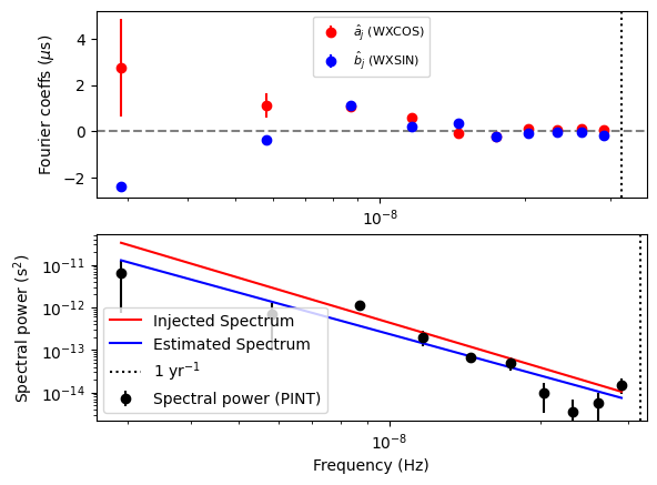
Note the outlier in the 1 year^-1 bin. This is caused by the covariance with RA and DEC, which introduce a delay with the same frequency.
DM noise fitting
Let us now do a similar kind of analysis for DM noise.
[11]:
par_sim = """
    PSR           SIM4
    RAJ           05:00:00     1
    DECJ          15:00:00     1
    PEPOCH        55000
    F0            100          1
    F1            -1e-15       1
    PHOFF         0            1
    DM            15           1
    TNDMAMP       -13
    TNDMGAM       3.5
    TNDMC         30
    TZRMJD        55000
    TZRFRQ        1400
    TZRSITE       gbt
    UNITS         TDB
    EPHEM         DE440
    CLOCK         TT(BIPM2019)
"""

m = get_model(StringIO(par_sim))
[12]:
# Generate the simulated TOAs.
ntoas = 2000
toaerrs = np.random.uniform(0.5, 2.0, ntoas) * u.us
freqs = np.linspace(500, 1500, 8) * u.MHz

t = make_fake_toas_uniform(
    startMJD=53001,
    endMJD=57001,
    ntoas=ntoas,
    model=m,
    freq=freqs,
    obs="gbt",
    error=toaerrs,
    add_noise=True,
    add_correlated_noise=True,
    name="fake",
    include_bipm=True,
    include_gps=True,
    multi_freqs_in_epoch=True,
)
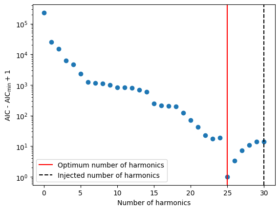
[13]:
# Find the optimum number of harmonics by minimizing AIC.
m1 = deepcopy(m)
m1.remove_component("PLDMNoise")

m2 = deepcopy(m1)

nharm_opt, d_aics = find_optimal_nharms(m2, t, "DMWaveX", 30)
print("Optimum no of harmonics = ", nharm_opt)
Optimum no of harmonics = 30
[14]:
# The Y axis is plotted in log scale only for better visibility.
plt.scatter(list(range(len(d_aics))), d_aics + 1)
plt.axvline(nharm_opt, color="red", label="Optimum number of harmonics")
plt.axvline(
    int(m.TNDMC.value), color="black", ls="--", label="Injected number of harmonics"
)
plt.xlabel("Number of harmonics")
plt.ylabel("AIC - AIC$_\\min{} + 1$")
plt.legend()
plt.yscale("log")
# plt.savefig("sim3-aic.pdf")
[15]:
# Now create a new model with the optimum number of
# harmonics
m2 = deepcopy(m1)

Tspan = t.get_mjds().max() - t.get_mjds().min()
dmwavex_setup(m2, T_span=Tspan, n_freqs=nharm_opt, freeze_params=False)

ftr = WLSFitter(t, m2)
ftr.fit_toas(maxiter=10)
m2 = ftr.model

print(m2)
# Created: 2024-05-02T16:06:37.969014
# PINT_version: 1.0+54.g0e607ed
# User: docs
# Host: build-24258979-project-85767-nanograv-pint
# OS: Linux-5.19.0-1028-aws-x86_64-with-glibc2.35
# Python: 3.11.6 (main, Feb  1 2024, 16:47:41) [GCC 11.4.0]
# Format: pint
PSR                                  SIM4
EPHEM                               DE440
CLOCK                        TT(BIPM2019)
UNITS                                 TDB
START              53000.9999999567933913
FINISH             56985.0000000470963310
DILATEFREQ                              N
DMDATA                                  N
NTOA                                 2000
CHI2                   1971.1115203337804
CHI2R                  1.0197162546993173
TRES                1.0004871879404677873
RAJ                      5:00:00.00000422 1 0.00000191519383133734
DECJ                    14:59:59.99997957 1 0.00016071879954330197
PMRA                                  0.0
PMDEC                                 0.0
PX                                    0.0
F0                 100.000000000000047094 1 3.677924536715014598e-14
F1               -9.99999429996255119e-16 1 8.282426390657092134e-22
PEPOCH             55000.0000000000000000
PLANET_SHAPIRO                          N
DM                  14.999992892620425964 1 4.8888067530853088514e-06
DMWXEPOCH          55000.0000000000000000
DMWXFREQ_0001       0.0002510040160585677
DMWXSIN_0001         0.004784432696479563 1 5.9608433044230135e-06
DMWXCOS_0001       -0.0020701710711931325 1 6.5945090384257316e-06
DMWXFREQ_0002       0.0005020080321171354
DMWXSIN_0002       -0.0002151868593995677 1 4.631239922972655e-06
DMWXCOS_0002        0.0006672364199749057 1 4.399411780002452e-06
DMWXFREQ_0003       0.0007530120481757032
DMWXSIN_0003      -0.00021604023233196928 1 4.372853292790847e-06
DMWXCOS_0003        -0.000729812432969959 1 4.291029428816e-06
DMWXFREQ_0004       0.0010040160642342708
DMWXSIN_0004       -5.908809238702459e-05 1 4.396702705141925e-06
DMWXCOS_0004       -0.0001284441765185486 1 4.181737444241144e-06
DMWXFREQ_0005       0.0012550200802928387
DMWXSIN_0005        0.0001841957594462948 1 4.306864875420353e-06
DMWXCOS_0005       0.00019004741443962893 1 4.2238166013350605e-06
DMWXFREQ_0006       0.0015060240963514064
DMWXSIN_0006       0.00010506191267328568 1 4.298760058450302e-06
DMWXCOS_0006       -8.583179491469642e-05 1 4.193105184188948e-06
DMWXFREQ_0007       0.0017570281124099742
DMWXSIN_0007        0.0001190916182627555 1 4.2767783340648995e-06
DMWXCOS_0007       -4.081589258631969e-05 1 4.208895339810137e-06
DMWXFREQ_0008       0.0020080321284685417
DMWXSIN_0008       0.00010029966887087978 1 4.302231133444963e-06
DMWXCOS_0008        6.038599065081691e-05 1 4.167100129781713e-06
DMWXFREQ_0009       0.0022590361445271098
DMWXSIN_0009       -3.235810677116201e-05 1 4.290208376311054e-06
DMWXCOS_0009       -3.068426585762246e-05 1 4.188673423408253e-06
DMWXFREQ_0010       0.0025100401605856774
DMWXSIN_0010      -4.0112820073472066e-05 1 4.222242692959873e-06
DMWXCOS_0010      -2.0535791598738445e-05 1 4.338908873352654e-06
DMWXFREQ_0011        0.002761044176644245
DMWXSIN_0011       -7.554544470005492e-05 1 6.789499623293527e-06
DMWXCOS_0011       -7.075012563769556e-05 1 6.901572166551911e-06
DMWXFREQ_0012       0.0030120481927028127
DMWXSIN_0012       -1.633251080813954e-05 1 4.27433220916863e-06
DMWXCOS_0012      -1.8783933995431607e-05 1 4.207576440222235e-06
DMWXFREQ_0013       0.0032630522087613804
DMWXSIN_0013      -2.2458047013499387e-05 1 4.1845619858112104e-06
DMWXCOS_0013        6.842471154080898e-06 1 4.278253321789589e-06
DMWXFREQ_0014       0.0035140562248199485
DMWXSIN_0014      -3.8478396078044365e-05 1 4.210056598165244e-06
DMWXCOS_0014        2.851713555829453e-05 1 4.24520104656374e-06
DMWXFREQ_0015        0.003765060240878516
DMWXSIN_0015       -4.197920462969455e-05 1 4.192390796538004e-06
DMWXCOS_0015       -3.364114449998145e-05 1 4.267581600577844e-06
DMWXFREQ_0016        0.004016064256937083
DMWXSIN_0016        2.966682098885399e-05 1 4.2892613833473216e-06
DMWXCOS_0016        -7.63082183855059e-06 1 4.163436310734253e-06
DMWXFREQ_0017        0.004267068272995652
DMWXSIN_0017      -2.8523496939134686e-05 1 4.237765400705771e-06
DMWXCOS_0017       -7.535686584559696e-06 1 4.219315505193638e-06
DMWXFREQ_0018       0.0045180722890542195
DMWXSIN_0018       -8.321536599350788e-06 1 4.267410098869098e-06
DMWXCOS_0018       1.0527192645439128e-06 1 4.196931114909494e-06
DMWXFREQ_0019        0.004769076305112787
DMWXSIN_0019       1.5045160307102342e-05 1 4.2629076134210345e-06
DMWXCOS_0019      -2.5794399645040813e-05 1 4.193437351616618e-06
DMWXFREQ_0020        0.005020080321171355
DMWXSIN_0020       2.9036849558188502e-05 1 4.215839274535906e-06
DMWXCOS_0020       1.1749032665739599e-05 1 4.249124447083484e-06
DMWXFREQ_0021       0.0052710843372299225
DMWXSIN_0021        4.673534589649611e-06 1 4.3280221129121635e-06
DMWXCOS_0021        6.140856969891847e-06 1 4.132987608651971e-06
DMWXFREQ_0022         0.00552208835328849
DMWXSIN_0022         -5.4401258928555e-06 1 4.25364137450981e-06
DMWXCOS_0022      -1.1546888230350273e-05 1 4.217292884197121e-06
DMWXFREQ_0023        0.005773092369347058
DMWXSIN_0023        8.714297354117749e-06 1 4.2675784527202946e-06
DMWXCOS_0023       1.9103373469970348e-06 1 4.199208957197699e-06
DMWXFREQ_0024       0.0060240963854056254
DMWXSIN_0024       -7.361978125662888e-06 1 4.256721297018583e-06
DMWXCOS_0024      -1.3178900123540535e-07 1 4.210376245826402e-06
DMWXFREQ_0025        0.006275100401464193
DMWXSIN_0025       -7.863110893271246e-06 1 4.249319639860948e-06
DMWXCOS_0025       1.6758575591721533e-07 1 4.212037381818677e-06
DMWXFREQ_0026        0.006526104417522761
DMWXSIN_0026      -1.1616918523461777e-05 1 4.290363546015798e-06
DMWXCOS_0026        2.977989935023756e-05 1 4.178868618478103e-06
DMWXFREQ_0027        0.006777108433581329
DMWXSIN_0027       -6.921700101008301e-06 1 4.176379820254314e-06
DMWXCOS_0027       1.0698102469977588e-05 1 4.298188660911003e-06
DMWXFREQ_0028        0.007028112449639897
DMWXSIN_0028       3.3046800007363966e-05 1 4.258806820832094e-06
DMWXCOS_0028       1.2907251016112718e-05 1 4.223361008452143e-06
DMWXFREQ_0029        0.007279116465698465
DMWXSIN_0029      -1.4875084825331147e-05 1 4.232290162346857e-06
DMWXCOS_0029       -4.862136871371481e-06 1 4.24299875499507e-06
DMWXFREQ_0030        0.007530120481757032
DMWXSIN_0030      -1.0276476915932796e-05 1 4.20243641829311e-06
DMWXCOS_0030       3.4497579194968614e-06 1 4.277231825877769e-06
TZRMJD             55000.0000000000000000
TZRSITE                               gbt
TZRFRQ                             1400.0
PHOFF              -0.0004719283334695277 1 5.528398407307158e-06
Estimating the spectral parameters from the DMWaveX fit.
[16]:
# Get the Fourier amplitudes and powers and their uncertainties.
# Note that the `DMWaveX` amplitudes have the units of DM.
# We multiply them by a constant factor to convert them to dimensions
# of time so that they are consistent with `PLDMNoise`.
scale = DMconst / (1400 * u.MHz) ** 2

idxs = np.array(m2.components["DMWaveX"].get_indices())
a = np.array(
    [(scale * m2[f"DMWXSIN_{idx:04d}"].quantity).to_value("s") for idx in idxs]
)
da = np.array(
    [(scale * m2[f"DMWXSIN_{idx:04d}"].uncertainty).to_value("s") for idx in idxs]
)
b = np.array(
    [(scale * m2[f"DMWXCOS_{idx:04d}"].quantity).to_value("s") for idx in idxs]
)
db = np.array(
    [(scale * m2[f"DMWXCOS_{idx:04d}"].uncertainty).to_value("s") for idx in idxs]
)
print(len(idxs))

P = (a**2 + b**2) / 2
dP = ((a * da) ** 2 + (b * db) ** 2) ** 0.5

f0 = (1 / Tspan).to_value(u.Hz)
fyr = (1 / u.year).to_value(u.Hz)
30
[17]:
# We can create a `PLDMNoise` model from the `DMWaveX` model.
# This will estimate the spectral parameters from the `DMWaveX`
# amplitudes.
m3 = pldmnoise_from_dmwavex(m2)
print(m3)
# Created: 2024-05-02T16:06:38.031908
# PINT_version: 1.0+54.g0e607ed
# User: docs
# Host: build-24258979-project-85767-nanograv-pint
# OS: Linux-5.19.0-1028-aws-x86_64-with-glibc2.35
# Python: 3.11.6 (main, Feb  1 2024, 16:47:41) [GCC 11.4.0]
# Format: pint
PSR                                  SIM4
EPHEM                               DE440
CLOCK                        TT(BIPM2019)
UNITS                                 TDB
START              53000.9999999567933913
FINISH             56985.0000000470963310
DILATEFREQ                              N
DMDATA                                  N
NTOA                                 2000
CHI2                   1971.1115203337804
CHI2R                  1.0197162546993173
TRES                1.0004871879404677873
RAJ                      5:00:00.00000422 1 0.00000191519383133734
DECJ                    14:59:59.99997957 1 0.00016071879954330197
PMRA                                  0.0
PMDEC                                 0.0
PX                                    0.0
F0                 100.000000000000047094 1 3.677924536715014598e-14
F1               -9.99999429996255119e-16 1 8.282426390657092134e-22
PEPOCH             55000.0000000000000000
PLANET_SHAPIRO                          N
DM                  14.999992892620425964 1 4.8888067530853088514e-06
TZRMJD             55000.0000000000000000
TZRSITE                               gbt
TZRFRQ                             1400.0
PHOFF              -0.0004719283334695277 1 5.528398407307158e-06
TNDMAMP               -12.936911815504295 0 0.04222323071628055
TNDMGAM                 3.296563514796768 0 0.19423551642629294
TNDMC                                30.0
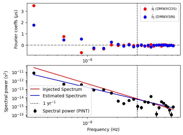
[18]:
# Now let us plot the estimated spectrum with the injected
# spectrum.
plt.subplot(211)
plt.errorbar(
    idxs * f0,
    b * 1e6,
    db * 1e6,
    ls="",
    marker="o",
    label="$\\hat{a}_j$ (DMWXCOS)",
    color="red",
)
plt.errorbar(
    idxs * f0,
    a * 1e6,
    da * 1e6,
    ls="",
    marker="o",
    label="$\\hat{b}_j$ (DMWXSIN)",
    color="blue",
)
plt.axvline(fyr, color="black", ls="dotted")
plt.axhline(0, color="grey", ls="--")
plt.ylabel("Fourier coeffs ($\mu$s)")
plt.xscale("log")
plt.legend(fontsize=8)

plt.subplot(212)
plt.errorbar(
    idxs * f0, P, dP, ls="", marker="o", label="Spectral power (PINT)", color="k"
)
P_inj = m.components["PLDMNoise"].get_noise_weights(t)[::2][:nharm_opt]
plt.plot(idxs * f0, P_inj, label="Injected Spectrum", color="r")
P_est = m3.components["PLDMNoise"].get_noise_weights(t)[::2][:nharm_opt]
print(len(idxs), len(P_est))
plt.plot(idxs * f0, P_est, label="Estimated Spectrum", color="b")
plt.xscale("log")
plt.yscale("log")
plt.ylabel("Spectral power (s$^2$)")
plt.xlabel("Frequency (Hz)")
plt.axvline(fyr, color="black", ls="dotted", label="1 yr$^{-1}$")
plt.legend()
30 30
[18]:
<matplotlib.legend.Legend at 0x7feb54d259d0>