This Jupyter notebook can be downloaded from PINT_walkthrough.ipynb, or viewed as a python script at PINT_walkthrough.py.
PINT Example Session
The PINT homepage is at: https://github.com/nanograv/PINT.
The documentation is availble here: https://nanograv-pint.readthedocs.io/en/latest/index.html
PINT can be run via a Python script, in an interactive session with ipython or jupyter, or using one of the command-line tools provided.
Times of Arrival (TOAs)
The raw data for PINT are TOAs, which can be read in from files in a variety of formats, or constructed programatically. PINT currently can read TEMPO, Tempo2, and ITOA text files, as well as a range of spacecraft FITS format event files (e.g. Fermi “FT1” and NICER .evt files).
Note: The first time TOAs get read in, lots of processing (can) happen, which can take some time. However, a “pickle” file can be saved, so the next time the same file is loaded (if nothing has changed), the TOAs will be loaded from the pickle file, which is much faster.
[1]:
import tempfile
import astropy.units as u
from pprint import pprint
from glob import glob
import pint.logging

# setup the logging
# let's have it give less detail
pint.logging.setup(level="WARNING")
[1]:
1
[2]:
%matplotlib inline
import matplotlib.pyplot as plt

# Turn on quantity support for plotting. This is very helpful!
from astropy.visualization import quantity_support

quantity_support()
[2]:
<astropy.visualization.units.quantity_support.<locals>.MplQuantityConverterFormatted at 0x799e05eb9090>
[3]:
# Here is how to create a single TOA in Python
# The first argument is an MJD(UTC) as a 2-double tuple to allow extended precision
# and the second argument is the TOA uncertainty
# Wherever possible, it is good to use astropy units on the values,
# but there are sensible defaults if you leave them out (us for uncertainty, MHz for freq)
import pint.toa as toa

a = toa.TOA(
    (54567, 0.876876876876876),
    4.5 * u.us,
    freq=1400.0 * u.MHz,
    obs="GBT",
    backend="GUPPI",
    name="guppi_56789.fits",
)
print(a)
54567.8768768768768759: 4.500 us error at 'gbt' at 1400.0000 MHz {'backend': 'GUPPI', 'name': 'guppi_56789.fits'}
[4]:
# An example of reading a TOA file
import pint.toa as toa
import pint.config

# maybe we want extra logging info here to see what happens when we load TOAs
pint.logging.setup(level="DEBUG")
t = toa.get_TOAs(pint.config.examplefile("NGC6440E.tim"), ephem="DE440")
# but then turn back to "WARNING" later
pint.logging.setup(level="WARNING")
DEBUG    (pint.toa                      ): No pulse number flags found in the TOAs
DEBUG    (pint.toa                      ): Applying clock corrections (include_bipm = True)
INFO     (pint.observatory              ): Applying GPS to UTC clock correction (~few nanoseconds)
DEBUG    (pint.observatory              ): Loading global GPS clock file
DEBUG    (pint.observatory.clock_file   ): Global clock file gps2utc.clk saving kwargs={'bogus_last_correction': False, 'valid_beyond_ends': False}
DEBUG    (pint.observatory.clock_file   ): Loading TEMPO2-format observatory clock correction file gps2utc.clk (/home/docs/.cache/astropy/download/url/d3c81b5766f4bfb84e65504c8a453085/contents) with bogus_last_correction=False
INFO     (pint.observatory              ): Using global clock file for gps2utc.clk with bogus_last_correction=False
INFO     (pint.observatory              ): Applying TT(TAI) to TT(BIPM2023) clock correction (~27 us)
INFO     (pint.observatory              ): Loading BIPM clock version bipm2023
DEBUG    (pint.observatory.clock_file   ): Global clock file tai2tt_bipm2023.clk saving kwargs={'bogus_last_correction': False, 'valid_beyond_ends': False}
DEBUG    (pint.observatory.clock_file   ): Loading TEMPO2-format observatory clock correction file tai2tt_bipm2023.clk (/home/docs/.cache/astropy/download/url/d0c6b0f6a57e39d4a167cd2aa08ad383/contents) with bogus_last_correction=False
INFO     (pint.observatory              ): Using global clock file for tai2tt_bipm2023.clk with bogus_last_correction=False
DEBUG    (pint.observatory.clock_file   ): Global clock file time_gbt.dat saving kwargs={'bogus_last_correction': False, 'valid_beyond_ends': False}
DEBUG    (pint.observatory.clock_file   ): Loading TEMPO-format observatory clock correction file time_gbt.dat (/home/docs/.cache/astropy/download/url/599e3ebbfc317e090244ee1ef4c79374/contents) with bogus_last_correction=False
INFO     (pint.observatory.clock_file   ): Disregarding suspicious MJD -2612.5 in TEMPO clock file
INFO     (pint.observatory              ): Using global clock file for time_gbt.dat with bogus_last_correction=False
INFO     (pint.observatory.topo_obs     ): Applying observatory clock corrections for observatory='gbt'.
DEBUG    (pint.toa                      ): Computing TDB columns.
DEBUG    (pint.toa                      ): Using EPHEM = DE440 for TDB calculation.
DEBUG    (pint.toa                      ): Computing PosVels of observatories and Earth, using DE440
INFO     (pint.solar_system_ephemerides ): Set solar system ephemeris to de440 through astropy
DEBUG    (pint.toa                      ): SSB obs pos [-1.31656418e+11 -6.52210907e+10 -2.82886126e+10] m
DEBUG    (pint.toa                      ): Adding columns ssb_obs_pos ssb_obs_vel obs_sun_pos
[4]:
3
[5]:
#  You can print a summary of the loaded TOAs
t.print_summary()
Number of TOAs:  62
Paradigm: narrowband
Number of commands:  0
Number of observatories: 1 ['gbt']
MJD span:  53478.286 to 54187.587
Date span: 2005-04-18 06:51:39.290648106 to 2007-03-28 14:05:44.808308037
gbt TOAs (62):
  Min freq:      1549.609 MHz
  Max freq:      2212.109 MHz
  Min error:     13.2 us
  Max error:     118 us
  Median error:  22.1 us
[6]:
# The get_mjds() method returns an array of the MJDs for the TOAs
# Here is the MJD of the first TOA. Notice that is has the units of days
pprint(t.get_mjds())
<Quantity [53478.28587142, 53483.27670519, 53489.46838979, 53679.87564592,
           53679.87564537, 53679.87564493, 53679.87564458, 53679.87564513,
           53681.700751  , 53681.9545449 , 53683.73678777, 53685.73745904,
           53687.68639838, 53687.95032739, 53690.8505221 , 53695.69557327,
           53695.85890789, 53700.71983242, 53700.86649642, 53709.63751695,
           53709.80961233, 53740.56747467, 53740.77459869, 53801.3860512 ,
           53801.59143301, 53833.2978103 , 53833.50245772, 53843.33207938,
           53865.18476778, 53865.37595138, 53895.11283426, 53895.3234694 ,
           53920.05274172, 53920.23971474, 53954.97216082, 53955.17456176,
           53980.90304181, 53981.11981343, 54010.82143311, 54011.03176787,
           54050.70474316, 54050.94624708, 54093.65660523, 54095.65330737,
           54098.6648706 , 54099.70978479, 54148.68651943, 54150.42513338,
           54151.52682219, 54152.71744732, 54153.54858413, 54160.52286339,
           54187.33158349, 54187.58732417, 54099.70978574, 54099.70978543,
           54099.70978515, 54099.7097849 , 54099.70978469, 54099.70978449,
           54099.70978432, 54099.70978416] d>
TOAs are stored in a Astropy Table in an instance of the TOAs class.
[7]:
# List the table columns, which include pre-computed TDB times and
# solar system positions and velocities
t.table.colnames
[7]:
['index',
 'mjd',
 'mjd_float',
 'error',
 'freq',
 'obs',
 'flags',
 'delta_pulse_number',
 'tdb',
 'tdbld',
 'ssb_obs_pos',
 'ssb_obs_vel',
 'obs_sun_pos']
Lots of cool things that tables can do…
[8]:
# This pops open a browser window showing the contents of the table
# t.table.show_in_browser()
Can do fancy sorting, selecting, re-arranging very easily.
[9]:
select = t.get_errors() < 20 * u.us
print(select)
[False False False False False False False  True False False False False
 False False  True False  True False False False  True False  True False
  True  True  True  True False  True False  True  True  True False False
 False False False False False False  True  True False  True  True False
 False False  True False False False False False False False False False
 False False]
[10]:
pprint(t.table["tdb"][select])
<Column name='tdb' dtype='object' length=18>
 53679.87638798794
 53690.85126495607
 53695.85965074819
 53709.81035518692
53740.775353131845
 53801.59218746964
  53833.2985647664
 53833.50321218054
 53843.33283383857
 53865.37670583518
 53895.32422385059
 53920.05349616944
53920.240469182434
 54093.65735966989
 54095.65406181057
 54099.71053923451
  54148.6872738913
 54153.54933858948
TOAs objects have a select() method to select based on a boolean mask. This selection can be undone later with unselect.
[11]:
t.print_summary()
t.select(select)
t.print_summary()
t.unselect()
t.print_summary()
Number of TOAs:  62
Paradigm: narrowband
Number of commands:  0
Number of observatories: 1 ['gbt']
MJD span:  53478.286 to 54187.587
Date span: 2005-04-18 06:51:39.290648106 to 2007-03-28 14:05:44.808308037
gbt TOAs (62):
  Min freq:      1549.609 MHz
  Max freq:      2212.109 MHz
  Min error:     13.2 us
  Max error:     118 us
  Median error:  22.1 us

Number of TOAs:  18
Paradigm: narrowband
Number of commands:  0
Number of observatories: 1 ['gbt']
MJD span:  53679.876 to 54153.549
Date span: 2005-11-05 21:00:55.739565465 to 2007-02-22 13:09:57.668850184
gbt TOAs (18):
  Min freq:      1949.609 MHz
  Max freq:      1949.609 MHz
  Min error:     13.2 us
  Max error:     19.6 us
  Median error:  16.4 us

Number of TOAs:  62
Paradigm: narrowband
Number of commands:  0
Number of observatories: 1 ['gbt']
MJD span:  53478.286 to 54187.587
Date span: 2005-04-18 06:51:39.290648106 to 2007-03-28 14:05:44.808308037
gbt TOAs (62):
  Min freq:      1549.609 MHz
  Max freq:      2212.109 MHz
  Min error:     13.2 us
  Max error:     118 us
  Median error:  22.1 us
PINT routines / classes / functions use Astropy Units internally and externally as much as possible:
[12]:
pprint(t.get_errors())
<Quantity [ 21.71,  21.95,  29.95,  25.46,  23.43,  31.67,  30.26,  13.52,
            21.64,  27.41,  24.58,  23.52,  21.71,  21.47,  17.72,  28.88,
            14.63,  38.03,  31.47,  33.26,  13.88,  26.89,  18.29,  21.48,
            17.88,  18.59,  19.03,  15.07,  21.58,  14.72,  25.14,  14.65,
            19.29,  13.25,  20.71,  23.57,  23.45,  22.16,  23.53,  21.01,
            21.66,  75.3 ,  19.65,  16.28,  21.93,  14.  ,  19.35,  32.92,
            33.83, 118.43,  16.45,  30.18,  21.8 ,  20.75,  32.75,  31.29,
            37.13,  37.4 ,  35.24,  50.83,  38.43,  48.59] us>
The times in each row contain (or are derived from) Astropy Time objects:
[13]:
toa0 = t.table["mjd"][0]
[14]:
toa0.tai
[14]:
<Time object: scale='tai' format='pulsar_mjd' value=53478.28624178991>
But the most useful timescale, TDB is also stored in its own column as a long double numpy array, to maintain precision and keep from having to redo the conversion. Note that is is the TOA time converted to the TDB timescale, but the Solar System delays have not been applied, so this is NOT what people call “barycentered times”
[15]:
pprint(t.table["tdbld"][:3])
<Column name='tdbld' dtype='float128' length=3>
53478.286614308378393
53483.277448077169023
53489.469132675783516
Timing Models
Now let’s define and load a timing model
[16]:
import pint.models as models

m = models.get_model(pint.config.examplefile("NGC6440E.par"))
[17]:
# Printing a model gives the parfile representation
print(m)
# Created: 2026-07-09T14:07:36.460324
# PINT_version: 0+untagged.346.g2f54939
# User: docs
# Host: build-33514996-project-85767-nanograv-pint
# OS: Linux-7.0.0-1004-aws-x86_64-with-glibc2.35
# Python: 3.11.15 (main, Jun 25 2026, 19:09:59) [GCC 11.4.0]
# Format: pint
# read_time: 2026-07-09T14:07:36.408962
# allow_tcb: False
# convert_tcb: False
# allow_T2: False
# original_name: /home/docs/checkouts/readthedocs.org/user_builds/nanograv-pint/envs/latest/lib/python3.11/site-packages/pint/data/examples/NGC6440E.par
PSR                            1748-2021E
EPHEM                               DE421
CLK                          TT(BIPM2019)
UNITS                                 TDB
TIMEEPH                              FB90
T2CMETHOD                        IAU2000B
DILATEFREQ                              N
DMDATA                                  N
NTOA                                    0
RAJ                     17:48:52.75000000 1 0.04999999999999999584
DECJ                   -20:21:29.00000000 1 0.40000000000000002220
PMRA                                  0.0
PMDEC                                 0.0
PX                                    0.0
POSEPOCH           53750.0000000000000000
F0                           61.485476554 1 5e-10
F1                             -1.181e-15 1 1e-18
PEPOCH             53750.0000000000000000
CORRECT_TROPOSPHERE                         N
PLANET_SHAPIRO                          N
SOLARN0                               0.0
NE_SW1                                0.0
SWM                                     0
DM                                  223.9 1 0.3
TZRMJD             53801.3860512007484954
TZRSITE                                 1
TZRFRQ                           1949.609
Timing models are composed of “delay” terms and “phase” terms, which are computed by the Components of the model. The delay terms are evaluated in order, going from terms local to the Solar System, which are needed for computing ‘barycenter-corrected’ TOAs, through terms for the binary system.
[18]:
# delay_funcs lists all the delay functions in the model, and the order is important!
m.delay_funcs
[18]:
[<bound method Astrometry.solar_system_geometric_delay of AstrometryEquatorial(
     MJDParameter(   POSEPOCH            53750.0000000000000000 (d) frozen=True),
     floatParameter( PX                  0.0               (mas) frozen=True),
     floatParameter( VLBIAX              UNSET,
     floatParameter( VLBIAY              UNSET,
     floatParameter( VLBIAZ              UNSET,
     AngleParameter( RAJ                 17:48:52.75000000 (hourangle) +/- 0h00m00.05s frozen=False),
     AngleParameter( DECJ                -20:21:29.00000000 (deg) +/- 0d00m00.4s frozen=False),
     floatParameter( PMRA                0.0               (mas / yr) frozen=True),
     floatParameter( PMDEC               0.0               (mas / yr) frozen=True))>,
 <bound method TroposphereDelay.troposphere_delay of TroposphereDelay(
     boolParameter(  CORRECT_TROPOSPHERE N                 frozen=True))>,
 <bound method SolarSystemShapiro.solar_system_shapiro_delay of SolarSystemShapiro(
     boolParameter(  PLANET_SHAPIRO      N                 frozen=True))>,
 <bound method SolarWindDispersion.solar_wind_delay of SolarWindDispersion(
     floatParameter( NE_SW               0.0               (1 / cm3) frozen=True),
     floatParameter( NE_SW1              0.0               (1 / (yr cm3)) frozen=True),
     MJDParameter(   SWEPOCH             UNSET,
     floatParameter( SWP                 2.0               () frozen=True),
     intParameter(   SWM                 0                 frozen=True))>,
 <bound method DispersionDM.constant_dispersion_delay of DispersionDM(
     floatParameter( DM                  223.9             (pc / cm3) +/- 0.3 pc / cm3 frozen=False),
     floatParameter( DM1                 UNSET,
     MJDParameter(   DMEPOCH             UNSET)>]
The phase functions include the spindown model and an absolute phase definition (if the TZR parameters are specified).
[19]:
# And phase_funcs holds a list of all the phase functions
m.phase_funcs
[19]:
[<bound method Spindown.spindown_phase of Spindown(
     floatParameter( F0                  61.485476554      (Hz) +/- 5e-10 Hz frozen=False),
     MJDParameter(   PEPOCH              53750.0000000000000000 (d) frozen=True),
     floatParameter( F1                  -1.181e-15        (Hz / s) +/- 1e-18 Hz / s frozen=False))>]
You can easily show/compute individual terms…
[20]:
ds = m.solar_system_shapiro_delay(t)
pprint(ds)
<Quantity [-4.11774615e-06, -4.58215733e-06, -5.09435415e-06,
            1.26025166e-05,  1.26025164e-05,  1.26025162e-05,
            1.26025160e-05,  1.26025163e-05,  1.34033282e-05,
            1.35163227e-05,  1.43416919e-05,  1.53159181e-05,
            1.63198995e-05,  1.64587639e-05,  1.80783671e-05,
            2.11530227e-05,  2.12647452e-05,  2.49851393e-05,
            2.51080759e-05,  3.45107578e-05,  3.47450146e-05,
            3.00319035e-05,  2.98083009e-05,  2.11804876e-06,
            2.07541048e-06, -3.00762925e-06, -3.03173087e-06,
           -4.09655364e-06, -5.80849733e-06, -5.81983363e-06,
           -6.90339229e-06, -6.90646307e-06, -6.82672804e-06,
           -6.82292820e-06, -5.19141699e-06, -5.17650521e-06,
           -2.63564143e-06, -2.60880558e-06,  2.28385789e-06,
            2.32788087e-06,  1.51692739e-05,  1.52882687e-05,
            5.13321680e-05,  4.61456318e-05,  3.99876478e-05,
            3.82020217e-05,  6.59654820e-06,  6.09155453e-06,
            5.78124972e-06,  5.45386906e-06,  5.22873335e-06,
            3.47897241e-06, -1.52400083e-06, -1.56079047e-06,
            3.82020202e-05,  3.82020207e-05,  3.82020211e-05,
            3.82020215e-05,  3.82020219e-05,  3.82020222e-05,
            3.82020225e-05,  3.82020227e-05] s>
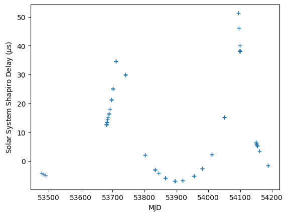
The get_mjds() method can return the TOA times as either astropy Time objects (for high precision), or as double precisions Quantities (for easy plotting).
[21]:
plt.plot(t.get_mjds(high_precision=False), ds.to(u.us), "+")
plt.xlabel("MJD")
plt.ylabel("Solar System Shapiro Delay ($\mu$s)")
[21]:
Text(0, 0.5, 'Solar System Shapiro Delay ($\\mu$s)')
Here are all of the terms added together:
[22]:
pprint(m.delay(t))
<Quantity [-256.27796452, -292.17743481, -333.75112984,  357.1520691 ,
            357.10408427,  357.06636421,  357.03617705,  357.08413648,
            367.69372882,  369.13822873,  379.08005434,  389.80438944,
            399.79826793,  401.11625247,  415.02771298,  435.8981066 ,
            436.5464231 ,  454.24090015,  454.72529413,  478.04191824,
            478.38369877,  468.46391764,  467.91545254,   94.36835601,
             92.628911  , -175.81800261, -177.4654317 , -253.52926427,
           -394.2164241 , -395.23707448, -497.24016588, -497.540425  ,
           -488.57121649, -488.17791764, -337.19445584, -335.91562337,
           -146.57400016, -144.80615177,  105.78789561,  107.54212818,
            389.24573948,  390.51810899,  490.40905135,  488.47319094,
            484.41349149,  482.68725532,  240.08971331,  226.85700881,
            218.50175843,  209.24129419,  202.56724193,  146.32198475,
            -81.97904962,  -84.14626638,  482.76923444,  482.74204028,
            482.71810824,  482.69693669,  482.67811686,  482.6613129 ,
            482.64624688,  482.63268713] s>
[23]:
pprint(m.phase(t))
Phase(int=<Quantity [-1.71639818e+09, -1.68988294e+09, -1.65698802e+09,
           -6.45521434e+08, -6.45521434e+08, -6.45521434e+08,
           -6.45521434e+08, -6.45521434e+08, -6.35826494e+08,
           -6.34478342e+08, -6.25011064e+08, -6.14383467e+08,
           -6.04030643e+08, -6.02628642e+08, -5.87222662e+08,
           -5.61485361e+08, -5.60617711e+08, -5.34795890e+08,
           -5.34016790e+08, -4.87423535e+08, -4.86509326e+08,
           -3.23112273e+08, -3.22011925e+08,  0.00000000e+00,
            1.09116600e+06,  1.69542892e+08,  1.70630151e+08,
            2.22853171e+08,  3.38950845e+08,  3.39966541e+08,
            4.97945399e+08,  4.99064384e+08,  6.30434263e+08,
            6.31427504e+08,  8.15928963e+08,  8.17004108e+08,
            9.53671033e+08,  9.54822490e+08,  1.11259234e+09,
            1.11370960e+09,  1.32444882e+09,  1.32573169e+09,
            1.55261772e+09,  1.56322501e+09,  1.57922372e+09,
            1.58477477e+09,  1.84497101e+09,  1.85420794e+09,
            1.86006100e+09,  1.86638658e+09,  1.87080228e+09,
            1.90785552e+09,  2.05028673e+09,  2.05164544e+09,
            1.58477477e+09,  1.58477477e+09,  1.58477477e+09,
            1.58477477e+09,  1.58477477e+09,  1.58477477e+09,
            1.58477477e+09,  1.58477477e+09]>, frac=<Quantity [-0.00309252, -0.00801063, -0.0171438 , -0.16868086, -0.16915065,
           -0.17547523, -0.17560751, -0.17249322, -0.16943038, -0.16625714,
           -0.16672537, -0.16423417, -0.16116986, -0.16013094, -0.15483818,
           -0.14701759, -0.1468638 , -0.13713971, -0.13910141, -0.12596384,
           -0.12321319, -0.06663884, -0.06750514, -0.00067575,  0.00150531,
           -0.00503603, -0.00931584, -0.01609301, -0.04283737, -0.04080684,
           -0.0929814 , -0.09457692, -0.13884716, -0.13800694, -0.18976956,
           -0.1910674 , -0.2118581 , -0.21299342, -0.21584403, -0.21263116,
           -0.17415625, -0.17657797, -0.09980529, -0.09705824, -0.09214972,
           -0.09090943, -0.02173754, -0.01961242, -0.01233623,  0.0003572 ,
           -0.01552563, -0.01669291, -0.01407142, -0.01213314, -0.08416629,
           -0.08750831, -0.09085623, -0.0897284 , -0.09223133, -0.08668348,
           -0.09712123, -0.09125008]>)
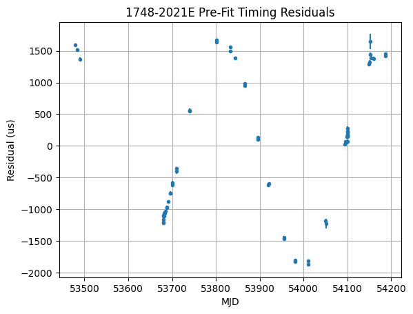
Residuals
[24]:
import pint.residuals
[25]:
rs = pint.residuals.Residuals(t, m)
[26]:
# Note that the Residuals object contains a toas member that has the TOAs used to compute
# the residuals, so you can use that to get the MJDs and uncertainties for each TOA
# Also note that plotting astropy Quantities must be enabled using
# astropy quanity_support() first (see beginning of this notebook)
plt.errorbar(
    rs.toas.get_mjds(),
    rs.time_resids.to(u.us),
    yerr=rs.toas.get_errors().to(u.us),
    fmt=".",
)
plt.title(f"{m.PSR.value} Pre-Fit Timing Residuals")
plt.xlabel("MJD")
plt.ylabel("Residual (us)")
plt.grid()
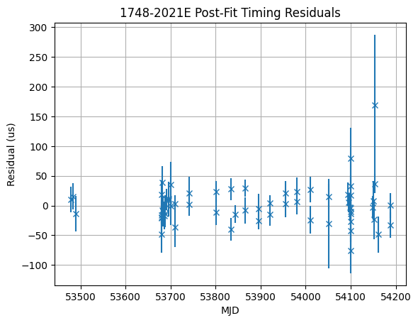
Fitting and Post-Fit residuals
The fitter is completely separate from the model and the TOA code. So you can use any type of fitter with some easy coding to create a new subclass of Fitter. This example uses PINT’s Weighted Least Squares fitter. The return value for this fitter is the chi^2 after the fit.
[27]:
import pint.fitter

f = pint.fitter.WLSFitter(t, m)
f.fit_toas()  # fit_toas() returns the final reduced chi squared
[27]:
np.longdouble('59.574367185473236685')
[28]:
# You can now print a nice human-readable summary of the fit
f.print_summary()
Fitted model using weighted_least_square method with 5 free parameters to 62 TOAs
Prefit residuals Wrms = 1090.793040947669 us, Postfit residuals Wrms = 21.18204717945037 us
Chisq = 59.574 for 56 d.o.f. for reduced Chisq of 1.064

PAR                        Prefit                  Postfit            Units
=================== ==================== ============================ =====
PSR                           1748-2021E 1748-2021E                   None
EPHEM                              DE421 DE440                        None
CLOCK                       TT(BIPM2019) TT(BIPM2023)                 None
UNITS                                TDB TDB                          None
START                                                         53478.3 d
FINISH                                                        54187.6 d
TIMEEPH                             FB90 FB90                         None
T2CMETHOD                       IAU2000B IAU2000B                     None
DILATEFREQ                             N                              None
DMDATA                                 N                              None
NTOA                                   0                              None
CHI2                                                          59.5744
CHI2R                                                         1.06383
TRES                                                           21.182 us
POSEPOCH                           53750                              d
PX                                     0                              mas
RAJ                         17h48m52.75s  17h48m52.80035401s +/- 0.00014 hourangle_second
DECJ                          -20d21m29s  -20d21m29.38334163s +/- 0.033 arcsec
PMRA                                   0                              mas / yr
PMDEC                                  0                              mas / yr
F0                               61.4855          61.485476554371(18) Hz
PEPOCH                             53750                              d
F1                            -1.181e-15            -1.1813(14)×10⁻¹⁵ Hz / s
CORRECT_TROPOSPHERE                    N                              None
PLANET_SHAPIRO                         N                              None
NE_SW                                  0                              1 / cm3
NE_SW1                                 0                              1 / (yr cm3)
SWP                                    2
SWM                                    0                              None
DM                                 223.9                  224.114(35) pc / cm3
TZRMJD                           53801.4                              d
TZRSITE                                1 1                            None
TZRFRQ                           1949.61                              MHz

Derived Parameters:
Period = 0.016264003404376±0.000000000000005 s
Pdot = (3.125±0.004)×10⁻¹⁹
Characteristic age = 8.246e+08 yr (braking index = 3)
Surface magnetic field = 2.28e+09 G
Magnetic field at light cylinder = 4881 G
Spindown Edot = 2.868e+33 erg / s (I=1e+45 cm2 g)
[29]:
# Lets plot the post-fit residuals
plt.errorbar(
    t.get_mjds(), f.resids.time_resids.to(u.us), t.get_errors().to(u.us), fmt="x"
)
plt.title(f"{m.PSR.value} Post-Fit Timing Residuals")
plt.xlabel("MJD")
plt.ylabel("Residual (us)")
plt.grid()
Now let’s save (and print) the post-fit par file. We’ll request a more TEMPO2-compatible file, though we could have requested a more TEMPO-style file or a more native PINT format. These differ only slightly, just as much as needed to be read by the three pieces of software. PINT can read all three variants.
[30]:
f.model.write_parfile("/tmp/output.par", format="tempo2")
print(f.model.as_parfile(format="tempo2"))
# Created: 2026-07-09T14:07:37.345902
# PINT_version: 0+untagged.346.g2f54939
# User: docs
# Host: build-33514996-project-85767-nanograv-pint
# OS: Linux-7.0.0-1004-aws-x86_64-with-glibc2.35
# Python: 3.11.15 (main, Jun 25 2026, 19:09:59) [GCC 11.4.0]
# Format: tempo2
# read_time: 2026-07-09T14:07:36.408962
# allow_tcb: False
# convert_tcb: False
# allow_T2: False
# original_name: /home/docs/checkouts/readthedocs.org/user_builds/nanograv-pint/envs/latest/lib/python3.11/site-packages/pint/data/examples/NGC6440E.par
MODE 1
PSR                            1748-2021E
EPHEM                               DE440
CLK                          TT(BIPM2023)
UNITS                                 TDB
START              53478.2858714195382639
FINISH             54187.5873241702319097
TIMEEPH                              FB90
#T2CMETHOD                        IAU2000B
DILATEFREQ                              N
DMDATA          0
NTOA                                   62
CHI2                   59.574367185473236
CHI2R                  1.0638279854548793
TRES                21.182047179450373357
RAJ                     17:48:52.80035401 1 0.00013524660895673348
DECJ                   -20:21:29.38334163 1 0.03285153305570395060
PMRA                                  0.0
PMDEC                                 0.0
PX                                    0.0
POSEPOCH           53750.0000000000000000
F0                  61.485476554371304245 1 1.8086084528481625616e-11
F1              -1.1813320788949692191e-15 1 1.4418540384438644559e-18
PEPOCH             53750.0000000000000000
CORRECT_TROPOSPHERE                         N
PLANET_SHAPIRO                          N
SOLARN0                               0.0
NE_SW1                                0.0
DM                  224.11379740488740489 1 0.034938980494124784182
TZRMJD             53801.3860512007484954
TZRSITE                                 1
TZRFRQ                           1949.609
Other interesting things
We can make Barycentered TOAs in a single line, if you have a model and a TOAs object! These are TDB times with the Solar System delays applied (precisely which of the delay components are applied is changeable – the default applies all delays before the ones associated with the binary system)
[31]:
pprint(m.get_barycentric_toas(t))
<Quantity [53478.28958049, 53483.28082976, 53489.47299554, 53679.87225507,
           53679.87225507, 53679.87225507, 53679.87225507, 53679.87225507,
           53681.69723814, 53681.95101532, 53683.73314312, 53685.73369027,
           53687.68251394, 53687.9464277 , 53690.84646139, 53695.69127101,
           53695.85459813, 53700.71531786, 53700.86197625, 53709.63272692,
           53709.80481834, 53740.56280708, 53740.76993744, 53801.38571344,
           53801.59111538, 53833.3005997 , 53833.50526618, 53843.33576821,
           53865.19008493, 53865.38128034, 53895.11934381, 53895.32998242,
           53920.05915093, 53920.24611939, 53954.97681797, 53955.1792041 ,
           53980.90549269, 53981.12224386, 54010.82096314, 54011.0312776 ,
           54050.70099243, 54050.94248163, 54093.65168364, 54095.64840819,
           54098.6600184 , 54099.70495258, 54148.68449508, 54150.42326217,
           54151.5250477 , 54152.71578   , 54153.54699406, 54160.52192431,
           54187.33328679, 54187.58905255, 54099.70495258, 54099.70495258,
           54099.70495258, 54099.70495258, 54099.70495258, 54099.70495258,
           54099.70495258, 54099.70495258] d>
Let’s export the clock corrections as they currently stand so we can save these exact versions for reproducibility purposes.
[32]:
import pint.observatory.topo_obs

d = tempfile.mkdtemp()
pint.observatory.topo_obs.export_all_clock_files(d)
for f in sorted(glob(f"{d}/*")):
    print(f)
/tmp/tmpyophew4p/gps2utc.clk
/tmp/tmpyophew4p/tai2tt_bipm2023.clk
/tmp/tmpyophew4p/time_gbt.dat