This Jupyter notebook can be downloaded from solar_wind.ipynb, or viewed as a python script at solar_wind.py.

Solar Wind Models

The standard solar wind model in PINT is implemented as the NE_SW parameter (Edwards et al. (2006)), which is the solar wind electron density at 1 AU (in cm\(^{-3}\)). This assumes that the electron density falls as \(r^{-2}\) away from the Sun. With SWM=0 this is all that is allowed.

However, in You et al. (2007) and You et al. (2012), they extend the model to other radial power-law indices \(r^{-p}\) (also see Hazboun et al. (2022)). This is now implemented with SWM=1 in PINT (and the power-law index is SWP).

Finally, it is clear that the solar wind model can vary from year to year (or even over shorter timescales). Therefore we now have a new SWX model (like DMX) that implements a separate solar wind model over different time intervals.

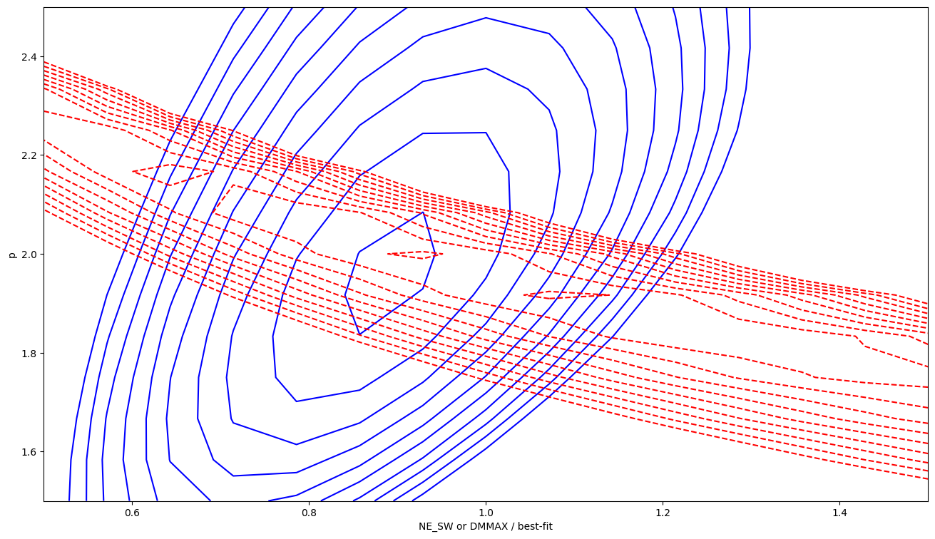
With the new model, though, there is covariance between the power-law index SWP and NE_SW, since most of the fit is determined by the maximum excess DM in the data. Therefore for the SWX model we have reparameterized it to use SWXDM: the max DM at conjunction. This makes the covariance a lot less. And to ensure continuity, this is explicitly the excess DM, so the DM from the SWX model at opposition is 0.

from io import StringIO
import numpy as np

from astropy.time import Time
import astropy.coordinates
from pint.models import get_model
from pint.fitter import Fitter
from pint.simulation import make_fake_toas_uniform
import pint.utils
import pint.gridutils
import pint.logging

import matplotlib.pyplot as plt

pint.logging.setup(level="WARNING")

1

Demonstrate the change in covariance going from NE_SW to DMMAX

par = """
PSR J1234+5678
F0 1
DM 10
ELAT 3
ELONG 0
PEPOCH 54000
EPHEM DE440
"""

# basic model using standard SW
model0 = get_model(StringIO("\n".join([par, "NE_SW 30\nSWM 0"])))

toas = pint.simulation.make_fake_toas_uniform(
    54000,
    54000 + 365,
    153,
    model=model0,
    obs="gbt",
    add_noise=True,
)

# standard model with variable index
model1 = get_model(StringIO("\n".join([par, "NE_SW 30\nSWM 1\nSWP 2"])))
# SWX model with 1 segment
model2 = get_model(
    StringIO(
        "\n".join(
            [par, "SWXDM_0001 1\nSWXP_0001 2\nSWXR1_0001 53999\nSWXR2_0001 55000"]
        )
    )
)
model2.SWXDM_0001.quantity = model0.get_max_dm()

# parameter grids
p = np.linspace(1.5, 2.5, 13)

ne_sw = model0.NE_SW.quantity * np.linspace(0.5, 1.5, 15)
dmmax = np.linspace(0.5, 1.5, len(ne_sw)) * model0.get_max_dm()

f1 = Fitter.auto(toas, model1)
chi2_SWM1 = pint.gridutils.grid_chisq(f1, ("NE_SW", "SWP"), (ne_sw, p))[0]

f2 = Fitter.auto(toas, model2)
chi2_SWX = pint.gridutils.grid_chisq(f2, ("SWXDM_0001", "SWXP_0001"), (dmmax, p))[0]

fig, ax = plt.subplots(figsize=(16, 9))
ax.contour(
    dmmax / model0.get_max_dm(),
    p,
    chi2_SWX - chi2_SWX.min(),
    np.linspace(2, 100, 10),
    colors="b",
)
ax.contour(
    ne_sw / model0.NE_SW.quantity,
    p,
    chi2_SWM1 - chi2_SWM1.min(),
    np.linspace(2, 100, 10),
    colors="r",
    linestyles="--",
)
ax.set_ylabel("p")
ax.set_xlabel("NE_SW or DMMAX / best-fit")

Text(0.5, 0, 'NE_SW or DMMAX / best-fit')

SW model limits & scalings

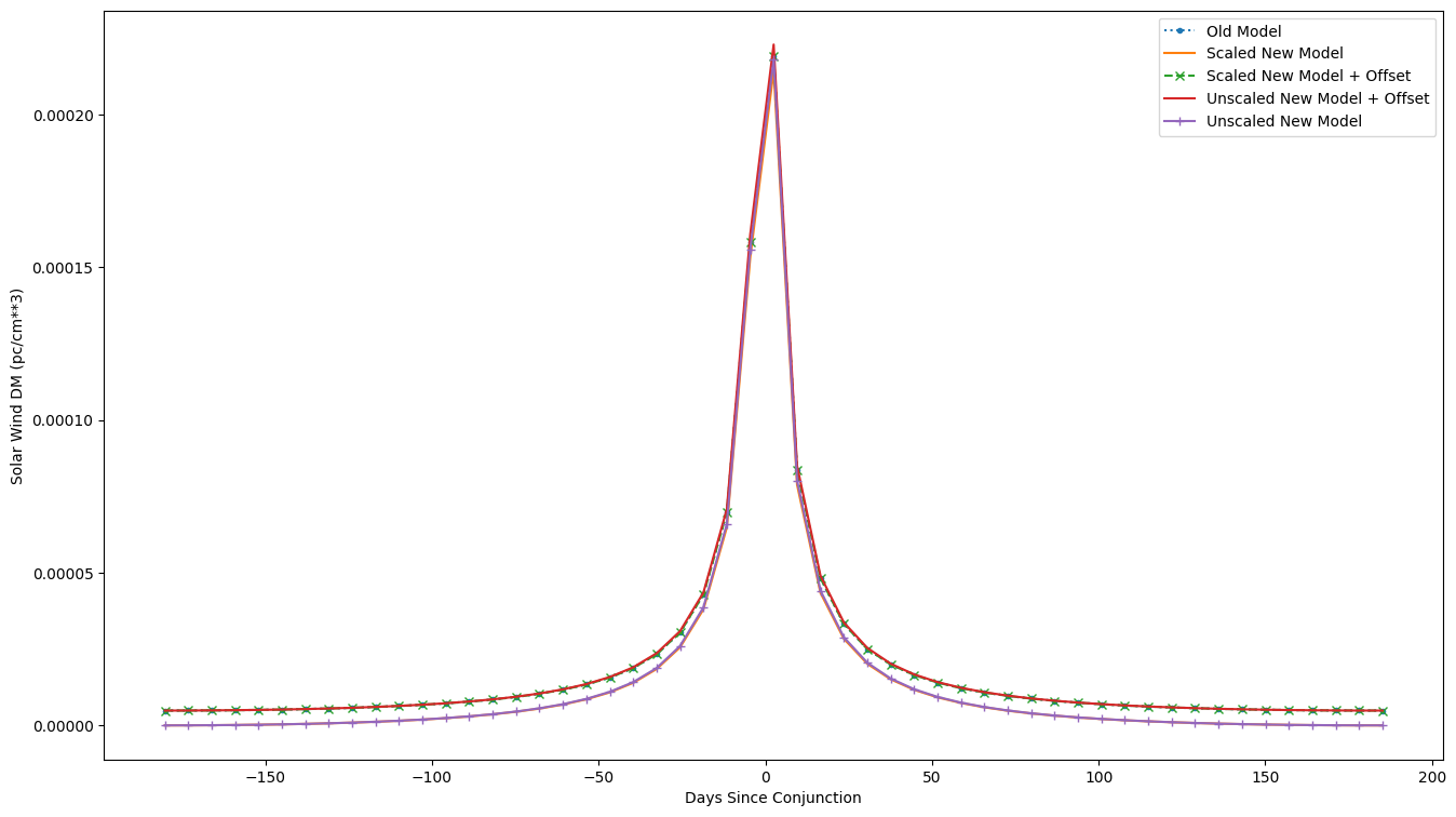
With the new SWX model, since it is only excess DM that starts at 0, in order to make the new model agree with the old you may need to scale some quantities

# default model
model = get_model(StringIO("\n".join([par, "NE_SW 1"])))
# SWX model with a single segment to match the default model
model2 = get_model(
    StringIO(
        "\n".join(
            [par, "SWXDM_0001 1\nSWXP_0001 2\nSWXR1_0001 53999\nSWXR2_0001 55000"]
        )
    )
)
# because of the way SWX is scaled, scale the input
scale = model2.get_swscalings()[0]
model2.SWXDM_0001.quantity = model.get_max_dm() * scale
toas = make_fake_toas_uniform(54000, 54000 + 365.25, 53, model=model, obs="gbt")

t0, elongation = pint.utils.get_conjunction(
    model.get_psr_coords(),
    Time(54000, format="mjd"),
    precision="high",
)

x = toas.get_mjds().value - t0.mjd
fig, ax = plt.subplots(figsize=(16, 9))
ax.plot(x, model.solar_wind_dm(toas), ".:", label="Old Model")
ax.plot(x, model2.swx_dm(toas), label="Scaled New Model")
ax.plot(
    x,
    model2.swx_dm(toas) + model.get_min_dm(),
    "x--",
    label="Scaled New Model + Offset",
)
model2.SWXDM_0001.quantity = model.get_max_dm()
ax.plot(
    x,
    model2.swx_dm(toas) + model.get_min_dm(),
    label="Unscaled New Model + Offset",
)
ax.plot(
    x,
    model2.swx_dm(toas),
    "+-",
    label="Unscaled New Model",
)
ax.set_xlabel("Days Since Conjunction")
ax.set_ylabel("Solar Wind DM (pc/cm**3)")
ax.legend()

<matplotlib.legend.Legend at 0x7fc98032cbd0>

Utility functions

A few functions to help move between models or separate model SWX segments

Find the next conjunction (time of SW max)

The low precision version just interpolates the Sun’s ecliptic longitude to match that of the pulsar. The high precision version uses better coordinate conversions to do this. It also returns the elongation at conjunction

t0, elongation = pint.utils.get_conjunction(
    model.get_psr_coords(),
    Time(54000, format="mjd"),
    precision="high",
)
print(f"Next conjunction at {t0}, with elongation {elongation}")

Next conjunction at 54180.109614738816, with elongation 2.9999638108834428 deg

As expected, the elongation is just about 3 degrees (the ecliptic latitude of the pulsar)

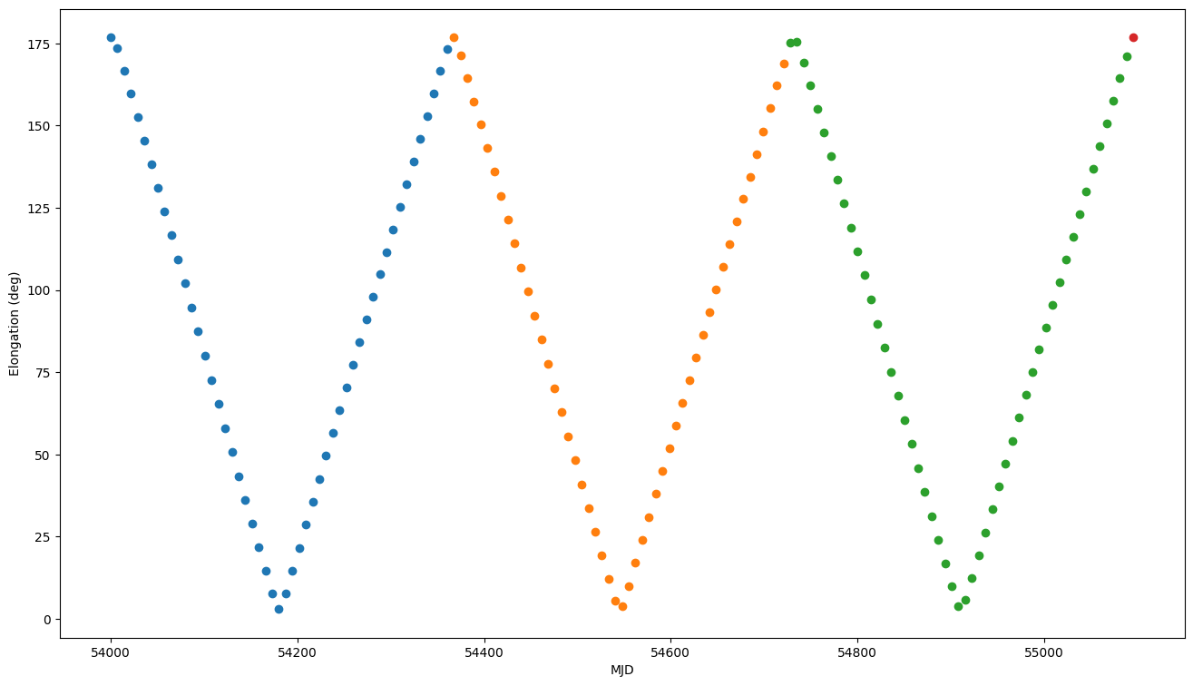
Divide the input times (TOAs) into years centered on each conjunction

This returns integer indices for each year

toas = make_fake_toas_uniform(54000, 54000 + 365.25 * 3, 153, model=model, obs="gbt")
elongation = astropy.coordinates.get_sun(
    Time(toas.get_mjds(), format="mjd")
).separation(model.get_psr_coords())
t0 = pint.utils.get_conjunction(
    model.get_psr_coords(), model.PEPOCH.quantity, precision="high"
)[0]
indices = pint.utils.divide_times(Time(toas.get_mjds(), format="mjd"), t0)
fig, ax = plt.subplots(figsize=(16, 9))
for i in np.unique(indices):
    ax.plot(toas.get_mjds()[indices == i], elongation[indices == i].value, "o")
ax.set_xlabel("MJD")
ax.set_ylabel("Elongation (deg)")

Text(0, 0.5, 'Elongation (deg)')

Get max/min DM from standard model, or NE_SW from SWX model

model0 = get_model(StringIO("\n".join([par, "NE_SW 30\nSWM 0"])))
# standard model with variable index
model1 = get_model(StringIO("\n".join([par, "NE_SW 30\nSWM 1\nSWP 2.5"])))
# SWX model with 1 segment
model2 = get_model(
    StringIO(
        "\n".join(
            [par, "SWXDM_0001 1\nSWXP_0001 2\nSWXR1_0001 53999\nSWXR2_0001 55000"]
        )
    )
)
# one value of the scale is returned for each SWX segment
scale = model2.get_swscalings()[0]
print(f"SW scaling: {scale}")
model2.SWXDM_0001.quantity = model0.get_max_dm() * scale

SW scaling: 0.9830510553813481

# Max is at conjunction, Min at opposition
print(
    f"SWM=0: NE_SW = {model0.NE_SW.quantity:.2f} Max DM = {model0.get_max_dm():.4f}, Min DM = {model0.get_min_dm():.4f}"
)
# Max and Min depend on NE_SW and SWP (covariance)
print(
    f"SWM=1 and SWP={model1.SWP.value}:  NE_SW = {model1.NE_SW.quantity:.2f} Max DM = {model1.get_max_dm():.4f}, Min DM = {model1.get_min_dm():.4f}"
)
# For SWX, the max/min values reported do not assume that it goes to 0 at opposition (for compatibility)
print(
    f"SWX and SWP={model2.SWXP_0001.value}: NE_SW = {model2.get_ne_sws()[0]:.2f} Max DM = {model2.get_max_dms()[0]:.4f}, Min DM = {model2.get_min_dms()[0]:.4f}"
)
print(
    f"SWX and SWP={model2.SWXP_0001.value}: Scaled NE_SW = {model2.get_ne_sws()[0]/scale:.2f} Scaled Max DM = {model2.get_max_dms()[0]/scale:.4f}, Scaled Min DM = {model2.get_min_dms()[0]/scale:.4f}"
)

SWM=0: NE_SW = 30.00 1 / cm3 Max DM = 0.0086 pc / cm3, Min DM = 0.0001 pc / cm3
SWM=1 and SWP=2.5:  NE_SW = 30.00 1 / cm3 Max DM = 0.0290 pc / cm3, Min DM = 0.0001 pc / cm3
SWX and SWP=2.0: NE_SW = 29.49 1 / cm3 Max DM = 0.0084 pc / cm3, Min DM = 0.0001 pc / cm3
SWX and SWP=2.0: Scaled NE_SW = 30.00 1 / cm3 Scaled Max DM = 0.0086 pc / cm3, Scaled Min DM = 0.0001 pc / cm3

The scaled values above agree between the SWM=0 and SWX models.