This Jupyter notebook can be downloaded from simulation_example.ipynb, or viewed as a python script at simulation_example.py.
Demonstrate TOA simulation using PINT
[1]:
from pint.models import get_model
from pint.simulation import (
    make_fake_toas_uniform,
    make_fake_toas_fromtim,
)
from pint.residuals import Residuals, WidebandTOAResiduals
from pint.logging import setup as setup_log
from pint import dmu
from pint.config import examplefile

import numpy as np
import matplotlib.pyplot as plt
import astropy.units as u
import io

# Turn logging level to warnings and above
setup_log(level="WARNING")
[1]:
1
Basic example
[2]:
# First, let us create a simple model from which we will simulate TOAs.
m = get_model(
    io.StringIO(
        """
        RAJ             05:00:00
        DECJ            20:00:00
        PEPOCH          55000
        F0              100
        F1              -1e-14
        DM              15
        PHOFF           0
        EFAC tel gbt    1.5
        TZRMJD          55000
        TZRFRQ          1400
        TZRSITE         gbt
        EPHEM           DE440
        CLOCK           TT(BIPM2019)
        UNITS           TDB
        """
    )
)
[3]:
# The simplest type of simulation we can do is narrowband TOAs with uniformly
# spaced epochs (one TOA per epoch) with a single frequency and equal TOA uncertainties.
tsim = make_fake_toas_uniform(
    model=m,
    startMJD=54000,
    endMJD=56000,
    ntoas=100,
    freq=1400 * u.MHz,
    obs="gbt",
    error=1 * u.us,
    include_bipm=True,
)
[4]:
# Let us try plotting the residuals
res = Residuals(tsim, m)

plt.errorbar(
    tsim.get_mjds(),
    res.time_resids.to_value("us"),
    res.get_data_error().to_value("us"),
    marker="+",
    ls="",
)
plt.xlabel("MJD")
plt.ylabel("Residuals (us)")
plt.show()
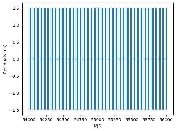
Here we see that the TOAs don’t have the expected white noise. The noise should be 1.5 us, including the EFAC. The noise can be included by using the add_noise option.
[5]:
tsim = make_fake_toas_uniform(
    model=m,
    startMJD=54000,
    endMJD=56000,
    ntoas=100,
    freq=1400 * u.MHz,
    obs="gbt",
    error=1 * u.us,
    include_bipm=True,
    add_noise=True,
)
[6]:
res = Residuals(tsim, m)

plt.errorbar(
    tsim.get_mjds(),
    res.time_resids.to_value("us"),
    res.get_data_error().to_value("us"),
    marker="+",
    ls="",
)
plt.xlabel("MJD")
plt.ylabel("Residuals (us)")
plt.show()
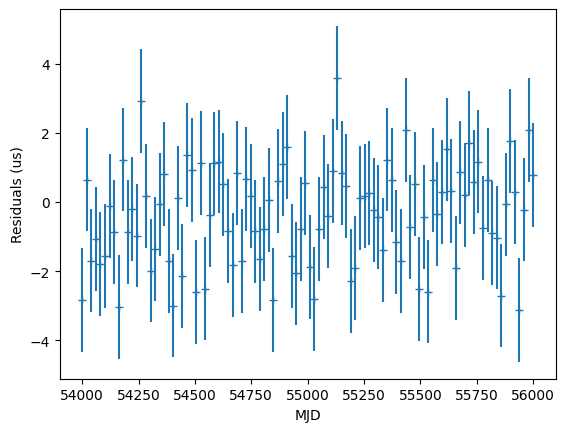
The same thing can be achieved in the command line using the following command:
$ zima --startMJD 54000 --ntoa 100 --duration 2000 --obs gbt --freq 1400 --error 1 --addnoise test.par test.tim
Multiple frequency example
Multiple frequency TOAs can be simulated by passing an array of frequencies into the freq parameter.
[7]:
freqs = np.linspace(1000, 2000, 4) * u.MHz
tsim = make_fake_toas_uniform(
    model=m,
    startMJD=54000,
    endMJD=56000,
    ntoas=100,
    freq=freqs,
    obs="gbt",
    error=1 * u.us,
    include_bipm=True,
    add_noise=True,
)
[8]:
res = Residuals(tsim, m)

plt.subplot(211)
plt.errorbar(
    tsim.get_mjds(),
    res.time_resids.to_value("us"),
    res.get_data_error().to_value("us"),
    marker="+",
    ls="",
)
plt.xlabel("MJD")
plt.ylabel("Residuals (us)")

plt.subplot(212)
plt.errorbar(
    tsim.get_freqs(),
    res.time_resids.to_value("us"),
    res.get_data_error().to_value("us"),
    marker="+",
    ls="",
)
plt.xlabel("Freq (MHz)")
plt.ylabel("Residuals (us)")
plt.show()
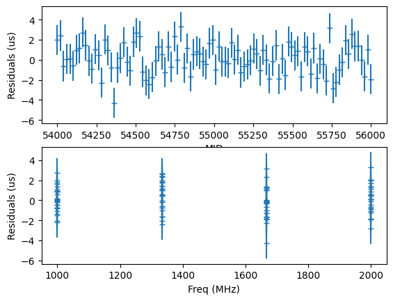
We see that the frequencies are distributed amongst epochs such that there is only one TOA per epoch. To distribute the TOAs such that each epoch contains all frequencies, use the multi_freqs_in_epoch option. Note that this option doesn’t change the total number of TOAs.
[9]:
freqs = np.linspace(1000, 2000, 4) * u.MHz
tsim = make_fake_toas_uniform(
    model=m,
    startMJD=54000,
    endMJD=56000,
    ntoas=100,
    freq=freqs,
    obs="gbt",
    error=1 * u.us,
    include_bipm=True,
    add_noise=True,
    multi_freqs_in_epoch=True,
)
[10]:
res = Residuals(tsim, m)

plt.subplot(211)
plt.errorbar(
    tsim.get_mjds(),
    res.time_resids.to_value("us"),
    res.get_data_error().to_value("us"),
    marker="+",
    ls="",
)
plt.xlabel("MJD")
plt.ylabel("Residuals (us)")

plt.subplot(212)
plt.errorbar(
    tsim.get_freqs(),
    res.time_resids.to_value("us"),
    res.get_data_error().to_value("us"),
    marker="+",
    ls="",
)
plt.xlabel("Freq(MHz)")
plt.ylabel("Residuals (us)")
plt.show()
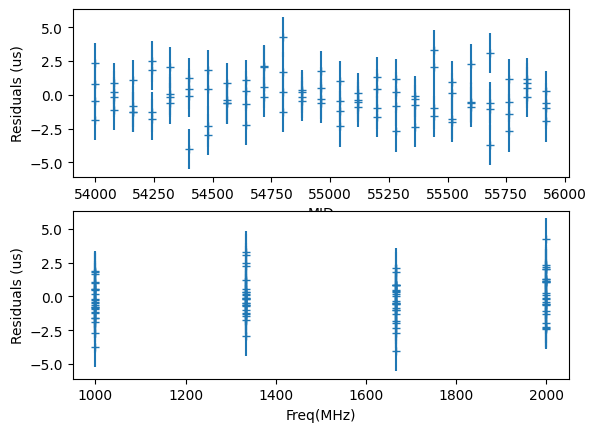
The same thing can be achieved in the command line using the following command:
$ zima --startMJD 54000 --ntoa 100 --duration 2000 --obs gbt --freq 1000 1333.33 1666.67 2000 --error 1 --addnoise --multifreq test.par test.tim
Correlated noise simulation example
If there is a correlated noise component in the timing model, an instance of that noise can be injected into the TOAs using the add_correlated_noise option.
[11]:
m1 = get_model(
    io.StringIO(
        """
        RAJ             05:00:00
        DECJ            20:00:00
        PEPOCH          55000
        F0              100
        F1              -1e-14
        DM              15
        PHOFF           0
        EFAC tel gbt    1.5
        TNREDAMP        -13
        TNREDGAM        4
        TZRMJD          55000
        TZRFRQ          1400
        TZRSITE         gbt
        EPHEM           DE440
        CLOCK           TT(BIPM2019)
        UNITS           TDB
        """
    )
)

tsim = make_fake_toas_uniform(
    model=m1,
    startMJD=54000,
    endMJD=56000,
    ntoas=100,
    freq=1400 * u.MHz,
    obs="gbt",
    error=1 * u.us,
    include_bipm=True,
    add_noise=True,
    add_correlated_noise=True,
)
[12]:
res = Residuals(tsim, m1)

plt.errorbar(
    tsim.get_mjds(),
    res.time_resids.to_value("us"),
    res.get_data_error().to_value("us"),
    marker="+",
    ls="",
)
plt.xlabel("MJD")
plt.ylabel("Residuals (us)")
plt.show()
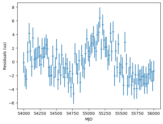
The same thing can be achieved in the command line using the following command:
$ zima --startMJD 54000 --ntoa 100 --duration 2000 --obs gbt --freq 1400 --error 1 --addnoise --addcorrnoise test.par test.tim
Wideband TOA simulation example
Wideband TOAs can be simulated using the wideband option. The white noise RMS for the wideband DMs is controlled using the wideband_dm_error parameter.
[13]:
m2 = get_model(
    io.StringIO(
        """
        RAJ             05:00:00
        DECJ            20:00:00
        PEPOCH          55000
        F0              100
        F1              -1e-14
        DMEPOCH         55000
        DM              15
        DM1             1
        DM2             0.5
        PHOFF           0
        EFAC tel gbt    1.5
        TZRMJD          55000
        TZRFRQ          1400
        TZRSITE         gbt
        EPHEM           DE440
        CLOCK           TT(BIPM2019)
        UNITS           TDB
        """
    )
)

tsim = make_fake_toas_uniform(
    model=m2,
    startMJD=54000,
    endMJD=56000,
    ntoas=100,
    freq=1400 * u.MHz,
    obs="gbt",
    error=1 * u.us,
    include_bipm=True,
    wideband=True,
    wideband_dm_error=1e-5 * dmu,
    add_noise=True,
)
[14]:
res = WidebandTOAResiduals(tsim, m2)

plt.subplot(211)
plt.errorbar(
    tsim.get_mjds(),
    res.toa.time_resids.to_value("us"),
    res.toa.get_data_error().to_value("us"),
    marker="+",
    ls="",
)
plt.xlabel("MJD")
plt.ylabel("Residuals (us)")

plt.subplot(212)
plt.errorbar(
    tsim.get_mjds(),
    tsim.get_dms().to_value(dmu),
    res.dm.get_data_error().to_value(dmu),
    marker="+",
    ls="",
)
plt.xlabel("MJD")
plt.ylabel("Wideband DM (dmu)")
plt.show()
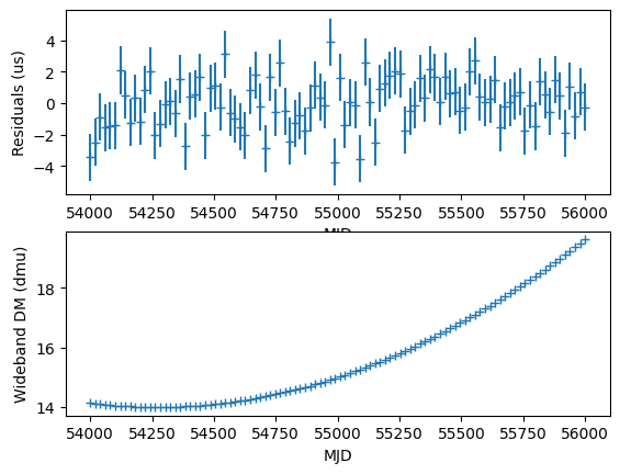
The same thing can be achieved in the command line using the following command:
::
$ zima –startMJD 54000 –ntoa 100 –duration 2000 –obs gbt –freq 1400 –error 1 –addnoise –wideband –dmerror 1e-5 test.par test.tim
Simulating TOAs based on a tim file
TOAs can be simulated to match the configuration of an existing tim file (e.g. epochs, TOA uncertainties, frequencies, flags, etc.) using the make_fake_toas_fromtim function. This also works with wideband tim files.
[15]:
tsim = make_fake_toas_fromtim(
    timfile=examplefile("B1855+09_NANOGrav_9yv1.tim"),
    model=m,
    add_noise=True,
)
WARNING (pint.logging ): /home/docs/checkouts/readthedocs.org/user_builds/nanograv-pint/envs/latest/lib/python3.11/site-packages/pint/models/noise_model.py:223 UserWarning: EFAC maskParameter(EFAC1 tel gbt 1.5 () frozen=True) has no TOAs
[16]:
res = Residuals(tsim, m)

plt.errorbar(
    tsim.get_mjds(),
    res.time_resids.to_value("us"),
    res.get_data_error().to_value("us"),
    marker="+",
    ls="",
)
plt.xlabel("MJD")
plt.ylabel("Residuals (us)")
plt.show()
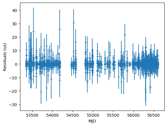
The same thing can be achieved in the command line using the following command:
::
$ zima –inputtim B1855+09_NANOGrav_9yv1.tim –addnoise test.par test.tim