This Jupyter notebook can be downloaded from noise-fitting-example.ipynb, or viewed as a python script at noise-fitting-example.py.
PINT Noise Fitting Examples
[1]:
from pint.models import get_model
from pint.simulation import make_fake_toas_uniform
from pint.logging import setup as setup_log
from pint.fitter import Fitter

import numpy as np
from io import StringIO
from astropy import units as u
from matplotlib import pyplot as plt
[2]:
setup_log(level="WARNING")
[2]:
1
Fitting for EFAC and EQUAD
[3]:
# Let us begin by simulating a dataset with an EFAC and an EQUAD.
# Note that the EFAC and the EQUAD are set as fit parameters ("1").
par = """
    PSR             TEST1
    RAJ             05:00:00    1
    DECJ            15:00:00    1
    PEPOCH          55000
    F0              100         1
    F1              -1e-15      1
    EFAC tel gbt    1.3         1
    EQUAD tel gbt   1.1         1
    TZRMJD          55000
    TZRFRQ          1400
    TZRSITE         gbt
    EPHEM           DE440
    CLOCK           TT(BIPM2019)
    UNITS           TDB
"""

m = get_model(StringIO(par))

ntoas = 200

# EFAC and EQUAD cannot be measured separately if all TOA uncertainties
# are the same. So we must set a different toa uncertainty for each TOA.
# This is how it is in real datasets anyway.
toaerrs = np.random.uniform(0.5, 2, ntoas) * u.us

t = make_fake_toas_uniform(
    startMJD=54000,
    endMJD=56000,
    ntoas=ntoas,
    model=m,
    obs="gbt",
    error=toaerrs,
    add_noise=True,
    include_bipm=True,
)
[4]:
# Now create the fitter. The `Fitter.auto()` function creates a
# Downhill fitter. Noise parameter fitting is only available in
# Downhill fitters.
ftr = Fitter.auto(t, m)
[5]:
# Now do the fitting.
ftr.fit_toas()
[6]:
# Print the post-fit model. We can see that the EFAC and EQUAD have been
# and the uncertainties are listed.
print(ftr.model)
# Created: 2026-07-21T01:49:52.798747
# PINT_version: 0+untagged.345.gd98e4eb
# User: docs
# Host: build-33679066-project-85767-nanograv-pint
# OS: Linux-7.0.0-1004-aws-x86_64-with-glibc2.35
# Python: 3.11.15 (main, Jun 25 2026, 19:09:59) [GCC 11.4.0]
# Format: pint
# read_time: 2026-07-21T01:49:49.015895
# allow_tcb: False
# convert_tcb: False
# allow_T2: False
PSR TEST1
EPHEM DE440
CLOCK TT(BIPM2019)
UNITS TDB
START 53999.9999999862546528
FINISH 56000.0000000056291204
DILATEFREQ N
DMDATA N
NTOA 200
CHI2 199.9999984424668
CHI2R 1.0362694219816933
TRES 1.9599216129731871
RAJ 4:59:59.99999791 1 0.00000704726447675635
DECJ 15:00:00.00031812 1 0.00061694855543327010
PMRA 0.0
PMDEC 0.0
PX 0.0
F0 100.00000000000018012 1 2.7236899860109183592e-13
F1 -1.0000039962094425787e-15 1 1.271178492576391023e-20
PEPOCH 55000.0000000000000000
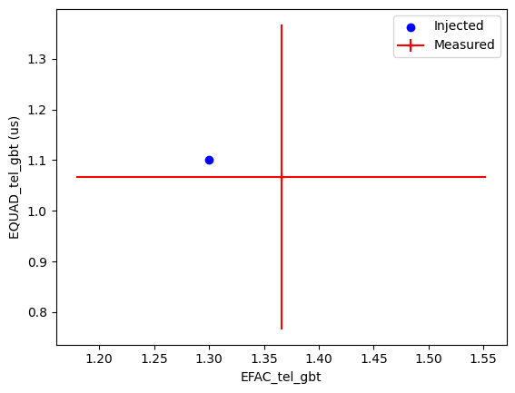
EFAC tel gbt 1.1615620881034239 1 0.1739804049702339
EQUAD tel gbt 1.1993406331237386 1 0.3351601304663429
TZRMJD 55000.0000000000000000
TZRSITE gbt
TZRFRQ 1400.0
PLANET_SHAPIRO N
[7]:
# Let us plot the injected and measured noise parameters together to
# compare them.
plt.scatter(m.EFAC1.value, m.EQUAD1.value, label="Injected", marker="o", color="blue")
plt.errorbar(
    ftr.model.EFAC1.value,
    ftr.model.EQUAD1.value,
    xerr=ftr.model.EFAC1.uncertainty_value,
    yerr=ftr.model.EQUAD1.uncertainty_value,
    marker="+",
    label="Measured",
    color="red",
)
plt.xlabel("EFAC_tel_gbt")
plt.ylabel("EQUAD_tel_gbt (us)")
plt.legend()
plt.show()
Fitting for ECORRs
[8]:
# Note the explicit offset (PHOFF) in the par file below.
# Implicit offset subtraction is typically not accurate enough when
# ECORR (or any other type of correlated noise) is present.
# i.e., PHOFF should be a free parameter when ECORRs are being fit.
par = """
    PSR             TEST2
    RAJ             05:00:00    1
    DECJ            15:00:00    1
    PEPOCH          55000
    F0              100         1
    F1              -1e-15      1
    PHOFF           0           1
    EFAC tel gbt    1.3         1
    ECORR tel gbt   1.1         1
    TZRMJD          55000
    TZRFRQ          1400
    TZRSITE         gbt
    EPHEM           DE440
    CLOCK           TT(BIPM2019)
    UNITS           TDB
"""

m = get_model(StringIO(par))

# ECORRs only apply when there are multiple TOAs per epoch.
# This can be simulated by providing multiple frequencies and
# setting the `multi_freqs_in_epoch` option. The `add_correlated_noise`
# option should also be set because correlated noise components
# are not simulated by default.

ntoas = 500
toaerrs = np.random.uniform(0.5, 2, ntoas) * u.us
freqs = np.linspace(1300, 1500, 4) * u.MHz

t = make_fake_toas_uniform(
    startMJD=54000,
    endMJD=56000,
    ntoas=ntoas,
    model=m,
    obs="gbt",
    error=toaerrs,
    freq=freqs,
    add_noise=True,
    add_correlated_noise=True,
    include_bipm=True,
    multi_freqs_in_epoch=True,
)
[9]:
ftr = Fitter.auto(t, m)
[10]:
ftr.fit_toas()
[10]:
True
[11]:
print(ftr.model)
# Created: 2026-07-21T01:50:01.809371
# PINT_version: 0+untagged.345.gd98e4eb
# User: docs
# Host: build-33679066-project-85767-nanograv-pint
# OS: Linux-7.0.0-1004-aws-x86_64-with-glibc2.35
# Python: 3.11.15 (main, Jun 25 2026, 19:09:59) [GCC 11.4.0]
# Format: pint
# read_time: 2026-07-21T01:49:52.932691
# allow_tcb: False
# convert_tcb: False
# allow_T2: False
PSR TEST2
EPHEM DE440
CLOCK TT(BIPM2019)
UNITS TDB
START 53999.9999999862155324
FINISH 55984.0000000565010764
DILATEFREQ N
DMDATA N
NTOA 500
CHI2 500.0044516029701
CHI2R 1.0162692105751425
TRES 1.7578057293869305
RAJ 4:59:59.99999149 1 0.00000645647222076328
DECJ 15:00:00.00018824 1 0.00055476402443504005
PMRA 0.0
PMDEC 0.0
PX 0.0
F0 99.99999999999985599 1 2.504067096429356942e-13
F1 -1.0000068356780675648e-15 1 1.14131940676339523046e-20
PEPOCH 55000.0000000000000000
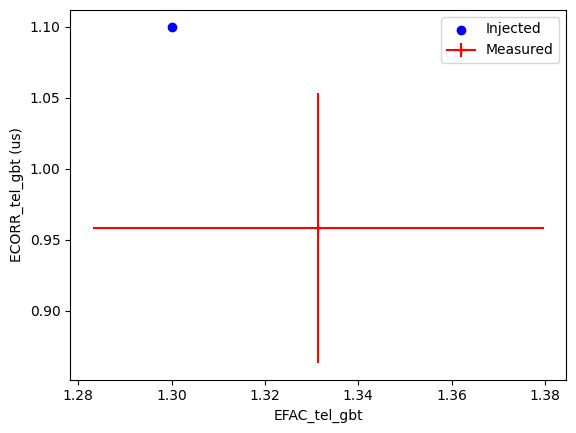
EFAC tel gbt 1.319015177272306 1 0.048326519386815744
ECORR tel gbt 1.216926165191393 1 0.10442920850083431
PLANET_SHAPIRO N
TZRMJD 55000.0000000000000000
TZRSITE gbt
TZRFRQ 1400.0
PHOFF -6.529698042525531e-06 1 1.8959647077596474e-05
[12]:
# Let us plot the injected and measured noise parameters together to
# compare them.
plt.scatter(m.EFAC1.value, m.ECORR1.value, label="Injected", marker="o", color="blue")
plt.errorbar(
    ftr.model.EFAC1.value,
    ftr.model.ECORR1.value,
    xerr=ftr.model.EFAC1.uncertainty_value,
    yerr=ftr.model.ECORR1.uncertainty_value,
    marker="+",
    label="Measured",
    color="red",
)
plt.xlabel("EFAC_tel_gbt")
plt.ylabel("ECORR_tel_gbt (us)")
plt.legend()
plt.show()