This Jupyter notebook can be downloaded from rednoise-fit-example.ipynb, or viewed as a python script at rednoise-fit-example.py.
Red noise, DM noise, and chromatic noise fitting examples
This notebook provides an example on how to fit for red noise and DM noise using PINT using simulated datasets.
We will use the PLRedNoise and PLDMNoise models to generate noise realizations (these models provide Fourier Gaussian process descriptions of achromatic red noise and DM noise respectively).
We will fit the generated datasets using the WaveX and DMWaveX models, which provide deterministic Fourier representations of achromatic red noise and DM noise respectively.
Finally, we will convert the WaveX/DMWaveX amplitudes into spectral parameters and compare them with the injected values.
[1]:
from pint import DMconst
from pint.models import get_model
from pint.simulation import make_fake_toas_uniform
from pint.logging import setup as setup_log
from pint.fitter import WLSFitter
from pint.utils import (
    cmwavex_setup,
    dmwavex_setup,
    find_optimal_nharms,
    plchromnoise_from_cmwavex,
    wavex_setup,
    plrednoise_from_wavex,
    pldmnoise_from_dmwavex,
)

from io import StringIO
import numpy as np
import astropy.units as u
from matplotlib import pyplot as plt
from copy import deepcopy

setup_log(level="WARNING")
[1]:
1
Red noise fitting
Simulation
The first step is to generate a simulated dataset for demonstration. Note that we are adding PHOFF as a free parameter. This is required for the fit to work properly.
[2]:
par_sim = """
    PSR           SIM3
    RAJ           05:00:00     1
    DECJ          15:00:00     1
    PEPOCH        55000
    F0            100          1
    F1            -1e-15       1
    PHOFF         0            1
    DM            15           1
    TNREDAMP      -13
    TNREDGAM      3.5
    TNREDC        30
    TZRMJD        55000
    TZRFRQ        1400
    TZRSITE       gbt
    UNITS         TDB
    EPHEM         DE440
    CLOCK         TT(BIPM2019)
"""

m = get_model(StringIO(par_sim))
[3]:
# Now generate the simulated TOAs.
ntoas = 2000
toaerrs = np.random.uniform(0.5, 2.0, ntoas) * u.us
freqs = np.linspace(500, 1500, 8) * u.MHz

t = make_fake_toas_uniform(
    startMJD=53001,
    endMJD=57001,
    ntoas=ntoas,
    model=m,
    freq=freqs,
    obs="gbt",
    error=toaerrs,
    add_noise=True,
    add_correlated_noise=True,
    name="fake",
    include_bipm=True,
    multi_freqs_in_epoch=True,
)
Optimal number of harmonics
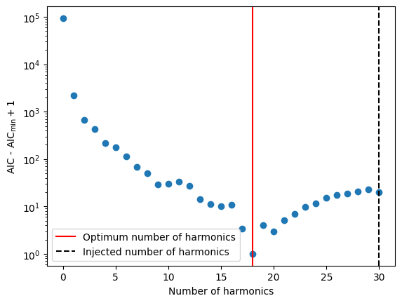
The optimal number of harmonics can be estimated by minimizing the Akaike Information Criterion (AIC). This is implemented in the pint.utils.find_optimal_nharms function.
[4]:
m1 = deepcopy(m)
m1.remove_component("PLRedNoise")

nharm_opt, d_aics = find_optimal_nharms(m1, t, "WaveX", 30)

print("Optimum no of harmonics = ", nharm_opt)
Optimum no of harmonics = 14
[5]:
print(np.argmin(d_aics))
14
[6]:
# The Y axis is plotted in log scale only for better visibility.
plt.scatter(list(range(len(d_aics))), d_aics + 1)
plt.axvline(nharm_opt, color="red", label="Optimum number of harmonics")
plt.axvline(
    int(m.TNREDC.value), color="black", ls="--", label="Injected number of harmonics"
)
plt.xlabel("Number of harmonics")
plt.ylabel("AIC - AIC$_\\min{} + 1$")
plt.legend()
plt.yscale("log")
# plt.savefig("sim3-aic.pdf")
[7]:
# Now create a new model with the optimum number of harmonics
m2 = deepcopy(m1)
Tspan = t.get_mjds().max() - t.get_mjds().min()
wavex_setup(m2, T_span=Tspan, n_freqs=nharm_opt, freeze_params=False)

ftr = WLSFitter(t, m2)
ftr.fit_toas(maxiter=10)
m2 = ftr.model

print(m2)
# Created: 2026-07-21T01:50:45.718996
# PINT_version: 0+untagged.345.gd98e4eb
# User: docs
# Host: build-33679066-project-85767-nanograv-pint
# OS: Linux-7.0.0-1004-aws-x86_64-with-glibc2.35
# Python: 3.11.15 (main, Jun 25 2026, 19:09:59) [GCC 11.4.0]
# Format: pint
# read_time: 2026-07-21T01:50:10.172948
# allow_tcb: False
# convert_tcb: False
# allow_T2: False
PSR                                  SIM3
EPHEM                               DE440
CLOCK                        TT(BIPM2019)
UNITS                                 TDB
START              53000.9999999567197106
FINISH             56985.0000000464631829
DILATEFREQ                              N
DMDATA                                  N
NTOA                                 2000
CHI2                   2029.7373729948886
CHI2R                  1.0329452279872207
TRES                   0.9969177076277939
RAJ                      5:00:00.00006706 1 0.00007718310507503812
DECJ                    14:59:59.98815938 1 0.00916737210621745673
PMRA                                  0.0
PMDEC                                 0.0
PX                                    0.0
F0                  100.00000000000019886 1 3.5971498552910960177e-13
F1              -9.997607631695820534e-16 1 1.5912163734269319623e-19
PEPOCH             55000.0000000000000000
PLANET_SHAPIRO                          N
DM                  14.999998964086807701 1 4.7608305386343749906e-06
WXEPOCH            55000.0000000000000000
WXFREQ_0001        0.00025100401605860305
WXSIN_0001         -4.689416422524177e-06 1 4.037020417728403e-07
WXCOS_0001        -1.5001025828184381e-05 1 9.609515117591319e-06
WXFREQ_0002         0.0005020080321172061
WXSIN_0002         1.9213553068512182e-07 1 2.0479569975714223e-07
WXCOS_0002         3.6610161016702326e-06 1 2.4394094591954647e-06
WXFREQ_0003         0.0007530120481758091
WXSIN_0003          2.127269184379038e-06 1 1.4322049790314823e-07
WXCOS_0003        -2.1438581631001404e-06 1 1.1150268841621723e-06
WXFREQ_0004         0.0010040160642344122
WXSIN_0004         1.1973328006882946e-07 1 1.14746650935969e-07
WXCOS_0004         1.0154404856682222e-06 1 6.547158983351552e-07
WXFREQ_0005         0.0012550200802930152
WXSIN_0005         -2.003366839628858e-07 1 1.0003553222661067e-07
WXCOS_0005         -5.415574315541952e-07 1 4.4657543799594334e-07
WXFREQ_0006         0.0015060240963516182
WXSIN_0006          7.485891753286175e-09 1 9.357089733330099e-08
WXCOS_0006          4.955635980157641e-07 1 3.373776413888274e-07
WXFREQ_0007         0.0017570281124102212
WXSIN_0007        -1.9683249474487593e-08 1 9.293817888407873e-08
WXCOS_0007         -5.519776027112086e-07 1 2.811294148123439e-07
WXFREQ_0008         0.0020080321284688244
WXSIN_0008          6.049904569133315e-08 1 9.896385492100506e-08
WXCOS_0008          5.315430335851523e-07 1 2.5769379085574533e-07
WXFREQ_0009          0.002259036144527427
WXSIN_0009         2.9636802366739444e-08 1 1.204097911231311e-07
WXCOS_0009         -3.632654313780044e-07 1 2.7514183623366855e-07
WXFREQ_0010         0.0025100401605860304
WXSIN_0010        -2.3159080215275805e-07 1 2.0308388604712616e-07
WXCOS_0010          5.040886668303353e-07 1 4.077649060194595e-07
WXFREQ_0011          0.002761044176644633
WXSIN_0011           7.52994012466516e-09 1 1.6342785398783134e-06
WXCOS_0011         3.6773693788142822e-06 1 2.844539284514134e-06
WXFREQ_0012         0.0030120481927032364
WXSIN_0012         -1.932984600350137e-08 1 1.20530418263184e-07
WXCOS_0012        -2.3507647621598087e-07 1 1.7512357433777518e-07
WXFREQ_0013         0.0032630522087618396
WXSIN_0013        -2.6126342332758837e-08 1 5.941794646492581e-08
WXCOS_0013        -1.7109118773987618e-08 1 7.149532899157776e-08
WXFREQ_0014         0.0035140562248204424
WXSIN_0014        -1.0246758489276164e-07 1 4.2644389304678204e-08
WXCOS_0014         -9.808004000918187e-08 1 4.4763808427859206e-08
TZRMJD             55000.0000000000000000
TZRSITE                               gbt
TZRFRQ                             1400.0
PHOFF             -0.00010429253683248872 1 0.00079448119901017
Estimating the spectral parameters from the WaveX fit.
[8]:
# Get the Fourier amplitudes and powers and their uncertainties.
idxs = np.array(m2.components["WaveX"].get_indices())
a = np.array([m2[f"WXSIN_{idx:04d}"].quantity.to_value("s") for idx in idxs])
da = np.array([m2[f"WXSIN_{idx:04d}"].uncertainty.to_value("s") for idx in idxs])
b = np.array([m2[f"WXCOS_{idx:04d}"].quantity.to_value("s") for idx in idxs])
db = np.array([m2[f"WXCOS_{idx:04d}"].uncertainty.to_value("s") for idx in idxs])
print(len(idxs))

P = (a**2 + b**2) / 2
dP = ((a * da) ** 2 + (b * db) ** 2) ** 0.5

f0 = (1 / Tspan).to_value(u.Hz)
fyr = (1 / u.year).to_value(u.Hz)
14
[9]:
# We can create a `PLRedNoise` model from the `WaveX` model.
# This will estimate the spectral parameters from the `WaveX`
# amplitudes.
m3 = plrednoise_from_wavex(m2)
print(m3)
# Created: 2026-07-21T01:50:45.748060
# PINT_version: 0+untagged.345.gd98e4eb
# User: docs
# Host: build-33679066-project-85767-nanograv-pint
# OS: Linux-7.0.0-1004-aws-x86_64-with-glibc2.35
# Python: 3.11.15 (main, Jun 25 2026, 19:09:59) [GCC 11.4.0]
# Format: pint
# read_time: 2026-07-21T01:50:10.172948
# allow_tcb: False
# convert_tcb: False
# allow_T2: False
PSR                                  SIM3
EPHEM                               DE440
CLOCK                        TT(BIPM2019)
UNITS                                 TDB
START              53000.9999999567197106
FINISH             56985.0000000464631829
DILATEFREQ                              N
DMDATA                                  N
NTOA                                 2000
CHI2                   2029.7373729948886
CHI2R                  1.0329452279872207
TRES                   0.9969177076277939
RAJ                      5:00:00.00006706 1 0.00007718310507503812
DECJ                    14:59:59.98815938 1 0.00916737210621745673
PMRA                                  0.0
PMDEC                                 0.0
PX                                    0.0
F0                  100.00000000000019886 1 3.5971498552910960177e-13
F1              -9.997607631695820534e-16 1 1.5912163734269319623e-19
PEPOCH             55000.0000000000000000
PLANET_SHAPIRO                          N
DM                  14.999998964086807701 1 4.7608305386343749906e-06
TZRMJD             55000.0000000000000000
TZRSITE                               gbt
TZRFRQ                             1400.0
PHOFF             -0.00010429253683248872 1 0.00079448119901017
TNREDAMP               -13.03759533272269 0 0.19179702427788195
TNREDGAM               3.9001232869952593 0 0.7309829560302343
TNREDC                                 14
[10]:
# Now let us plot the estimated spectrum with the injected
# spectrum.
plt.subplot(211)
plt.errorbar(
    idxs * f0,
    b * 1e6,
    db * 1e6,
    ls="",
    marker="o",
    label="$\\hat{a}_j$ (WXCOS)",
    color="red",
)
plt.errorbar(
    idxs * f0,
    a * 1e6,
    da * 1e6,
    ls="",
    marker="o",
    label="$\\hat{b}_j$ (WXSIN)",
    color="blue",
)
plt.axvline(fyr, color="black", ls="dotted")
plt.axhline(0, color="grey", ls="--")
plt.ylabel("Fourier coeffs ($\mu$s)")
plt.xscale("log")
plt.legend(fontsize=8)

plt.subplot(212)
plt.errorbar(
    idxs * f0, P, dP, ls="", marker="o", label="Spectral power (PINT)", color="k"
)
P_inj = m.components["PLRedNoise"].get_noise_weights(t)[::2][:nharm_opt]
plt.plot(idxs * f0, P_inj, label="Injected Spectrum", color="r")
P_est = m3.components["PLRedNoise"].get_noise_weights(t)[::2][:nharm_opt]
print(len(idxs), len(P_est))
plt.plot(idxs * f0, P_est, label="Estimated Spectrum", color="b")
plt.xscale("log")
plt.yscale("log")
plt.ylabel("Spectral power (s$^2$)")
plt.xlabel("Frequency (Hz)")
plt.axvline(fyr, color="black", ls="dotted", label="1 yr$^{-1}$")
plt.legend()
14 14
[10]:
<matplotlib.legend.Legend at 0x770fec123810>
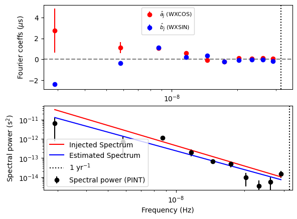
Note the outlier in the 1 year^-1 bin. This is caused by the covariance with RA and DEC, which introduce a delay with the same frequency.
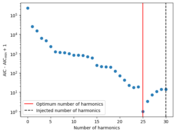
DM noise fitting
Let us now do a similar kind of analysis for DM noise.
[11]:
par_sim = """
    PSR           SIM4
    RAJ           05:00:00     1
    DECJ          15:00:00     1
    PEPOCH        55000
    F0            100          1
    F1            -1e-15       1
    PHOFF         0            1
    DM            15           1
    TNDMAMP       -13
    TNDMGAM       3.5
    TNDMC         30
    TZRMJD        55000
    TZRFRQ        1400
    TZRSITE       gbt
    UNITS         TDB
    EPHEM         DE440
    CLOCK         TT(BIPM2019)
"""

m = get_model(StringIO(par_sim))
[12]:
# Generate the simulated TOAs.
ntoas = 2000
toaerrs = np.random.uniform(0.5, 2.0, ntoas) * u.us
freqs = np.linspace(500, 1500, 8) * u.MHz

t = make_fake_toas_uniform(
    startMJD=53001,
    endMJD=57001,
    ntoas=ntoas,
    model=m,
    freq=freqs,
    obs="gbt",
    error=toaerrs,
    add_noise=True,
    add_correlated_noise=True,
    name="fake",
    include_bipm=True,
    multi_freqs_in_epoch=True,
)
[13]:
# Find the optimum number of harmonics by minimizing AIC.
m1 = deepcopy(m)
m1.remove_component("PLDMNoise")

m2 = deepcopy(m1)

nharm_opt, d_aics = find_optimal_nharms(m2, t, "DMWaveX", 30)
print("Optimum no of harmonics = ", nharm_opt)
Optimum no of harmonics = 30
[14]:
# The Y axis is plotted in log scale only for better visibility.
plt.scatter(list(range(len(d_aics))), d_aics + 1)
plt.axvline(nharm_opt, color="red", label="Optimum number of harmonics")
plt.axvline(
    int(m.TNDMC.value), color="black", ls="--", label="Injected number of harmonics"
)
plt.xlabel("Number of harmonics")
plt.ylabel("AIC - AIC$_\\min{} + 1$")
plt.legend()
plt.yscale("log")
# plt.savefig("sim3-aic.pdf")
[15]:
# Now create a new model with the optimum number of
# harmonics
m2 = deepcopy(m1)

Tspan = t.get_mjds().max() - t.get_mjds().min()
dmwavex_setup(m2, T_span=Tspan, n_freqs=nharm_opt, freeze_params=False)

ftr = WLSFitter(t, m2)
ftr.fit_toas(maxiter=10)
m2 = ftr.model

print(m2)
# Created: 2026-07-21T01:51:27.902578
# PINT_version: 0+untagged.345.gd98e4eb
# User: docs
# Host: build-33679066-project-85767-nanograv-pint
# OS: Linux-7.0.0-1004-aws-x86_64-with-glibc2.35
# Python: 3.11.15 (main, Jun 25 2026, 19:09:59) [GCC 11.4.0]
# Format: pint
# read_time: 2026-07-21T01:50:46.199221
# allow_tcb: False
# convert_tcb: False
# allow_T2: False
PSR                                  SIM4
EPHEM                               DE440
CLOCK                        TT(BIPM2019)
UNITS                                 TDB
START              53000.9999999567092824
FINISH             56985.0000000465434954
DILATEFREQ                              N
DMDATA                                  N
NTOA                                 2000
CHI2                   1926.0533498429536
CHI2R                   0.996406285485232
TRES                    0.983913914138379
RAJ                      4:59:59.99999946 1 0.00000190692577629606
DECJ                    15:00:00.00001782 1 0.00015996764830637916
PMRA                                  0.0
PMDEC                                 0.0
PX                                    0.0
F0                 100.000000000000050314 1 3.6221067063818455608e-14
F1              -9.999991981166614756e-16 1 8.4129217378770951107e-22
PEPOCH             55000.0000000000000000
PLANET_SHAPIRO                          N
DM                 14.9999985822129945435 1 4.983078983755504559e-06
DMWXEPOCH          55000.0000000000000000
DMWXFREQ_0001       0.0002510040160585971
DMWXSIN_0001       -0.0032967617725669115 1 5.977398329840956e-06
DMWXCOS_0001        0.0011708088120342157 1 6.988140503208355e-06
DMWXFREQ_0002       0.0005020080321171942
DMWXSIN_0002       -0.0004717621867972265 1 4.8689687521066e-06
DMWXCOS_0002        0.0005892039048242936 1 4.469149204317767e-06
DMWXFREQ_0003       0.0007530120481757912
DMWXSIN_0003       0.00020568626211840373 1 4.5791338141891145e-06
DMWXCOS_0003       -0.0010668925103932952 1 4.369037179516574e-06
DMWXFREQ_0004       0.0010040160642343884
DMWXSIN_0004        0.0006759711494064004 1 4.406587016270878e-06
DMWXCOS_0004       0.00010273006724458178 1 4.372662916714386e-06
DMWXFREQ_0005       0.0012550200802929853
DMWXSIN_0005      -0.00014430014110333202 1 4.305392622082963e-06
DMWXCOS_0005        1.858697874758961e-05 1 4.420467824804969e-06
DMWXFREQ_0006       0.0015060240963515824
DMWXSIN_0006        7.952605875667259e-05 1 4.295202383250851e-06
DMWXCOS_0006        6.261262020923473e-05 1 4.412007346043278e-06
DMWXFREQ_0007       0.0017570281124101796
DMWXSIN_0007        9.114597352766753e-05 1 4.3119318093619506e-06
DMWXCOS_0007       -3.716827319651395e-05 1 4.368432450344148e-06
DMWXFREQ_0008       0.0020080321284687767
DMWXSIN_0008       0.00010255528324805752 1 4.3693748350738955e-06
DMWXCOS_0008         6.26712545021116e-05 1 4.3095116747356445e-06
DMWXFREQ_0009        0.002259036144527374
DMWXSIN_0009       -6.457348862177071e-06 1 4.30545552208357e-06
DMWXCOS_0009       1.1796929393570318e-06 1 4.377239595361553e-06
DMWXFREQ_0010       0.0025100401605859706
DMWXSIN_0010        7.000641546938668e-05 1 4.425790905249351e-06
DMWXCOS_0010       1.3179646472739976e-05 1 4.314720892664313e-06
DMWXFREQ_0011       0.0027610441766445677
DMWXSIN_0011        2.364041882839511e-05 1 7.005356215077044e-06
DMWXCOS_0011         -2.6629976831876e-05 1 6.936697237589573e-06
DMWXFREQ_0012        0.003012048192703165
DMWXSIN_0012       -2.396780756289505e-05 1 4.309622107043417e-06
DMWXCOS_0012      -6.7267565542844975e-06 1 4.391407885641124e-06
DMWXFREQ_0013        0.003263052208761762
DMWXSIN_0013       1.6997538319720892e-06 1 4.344771748886362e-06
DMWXCOS_0013       1.5156178581944519e-05 1 4.336456896300952e-06
DMWXFREQ_0014        0.003514056224820359
DMWXSIN_0014        6.156963918259382e-05 1 4.257866543484252e-06
DMWXCOS_0014       -1.953623632954299e-05 1 4.403889947797256e-06
DMWXFREQ_0015       0.0037650602408789563
DMWXSIN_0015       -4.148409593546127e-05 1 4.4200959639629165e-06
DMWXCOS_0015       2.8803602823140342e-05 1 4.231206590263585e-06
DMWXFREQ_0016       0.0040160642569375534
DMWXSIN_0016        2.720730944675695e-06 1 4.3684746418554054e-06
DMWXCOS_0016       -1.710823150617997e-05 1 4.291626073805135e-06
DMWXFREQ_0017        0.004267068272996151
DMWXSIN_0017       -7.451484381154812e-06 1 4.308626347784441e-06
DMWXCOS_0017      -1.9761781094767838e-05 1 4.354426717112754e-06
DMWXFREQ_0018        0.004518072289054748
DMWXSIN_0018       -1.358654596395121e-05 1 4.251832370677451e-06
DMWXCOS_0018        7.114445791957062e-06 1 4.413517178214711e-06
DMWXFREQ_0019        0.004769076305113344
DMWXSIN_0019       -3.082043233023971e-06 1 4.302738561869708e-06
DMWXCOS_0019      -1.4152293690672768e-05 1 4.371679368887172e-06
DMWXFREQ_0020        0.005020080321171941
DMWXSIN_0020        5.865168959454808e-06 1 4.334261667990881e-06
DMWXCOS_0020      -1.9914302176677272e-05 1 4.337489649964175e-06
DMWXFREQ_0021        0.005271084337230538
DMWXSIN_0021      -1.3100674758353283e-06 1 4.277862132627315e-06
DMWXCOS_0021        4.072073895396388e-06 1 4.387998475641654e-06
DMWXFREQ_0022       0.0055220883532891354
DMWXSIN_0022       -4.542030775423394e-06 1 4.3154157509617745e-06
DMWXCOS_0022        2.337404599610422e-05 1 4.346699389743563e-06
DMWXFREQ_0023        0.005773092369347733
DMWXSIN_0023       -9.255340135389587e-06 1 4.2615316363825995e-06
DMWXCOS_0023       3.6921113592240483e-06 1 4.395000330967149e-06
DMWXFREQ_0024         0.00602409638540633
DMWXSIN_0024         7.93238537222578e-06 1 4.3046512692434176e-06
DMWXCOS_0024      -1.4900006111371303e-06 1 4.350886997146349e-06
DMWXFREQ_0025        0.006275100401464927
DMWXSIN_0025        3.226740343579094e-07 1 4.295514992033024e-06
DMWXCOS_0025       3.6314101938887477e-06 1 4.361750300860142e-06
DMWXFREQ_0026        0.006526104417523524
DMWXSIN_0026       1.2248582831768422e-05 1 4.326409192495347e-06
DMWXCOS_0026       -6.045935777650347e-06 1 4.320161743170583e-06
DMWXFREQ_0027        0.006777108433582121
DMWXSIN_0027       3.7706005870495502e-06 1 4.388801585300919e-06
DMWXCOS_0027       1.3962337759917482e-05 1 4.255230309927461e-06
DMWXFREQ_0028        0.007028112449640718
DMWXSIN_0028      -3.7978859233537535e-06 1 4.3881927129131265e-06
DMWXCOS_0028      -1.4937822985811946e-06 1 4.257207419127452e-06
DMWXFREQ_0029       0.0072791164656993155
DMWXSIN_0029       3.4990314841452993e-06 1 4.2975698858345715e-06
DMWXCOS_0029        8.237973165792199e-06 1 4.3443523553164e-06
DMWXFREQ_0030        0.007530120481757913
DMWXSIN_0030       -3.063488748395314e-06 1 4.3505175808073765e-06
DMWXCOS_0030        1.570799393094524e-05 1 4.288810962772396e-06
TZRMJD             55000.0000000000000000
TZRSITE                               gbt
TZRFRQ                             1400.0
PHOFF              0.00019104606932709718 1 5.5934863376331e-06
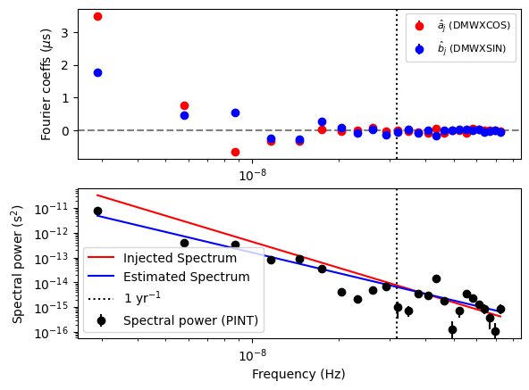
Estimating the spectral parameters from the DMWaveX fit.
[16]:
# Get the Fourier amplitudes and powers and their uncertainties.
# Note that the `DMWaveX` amplitudes have the units of DM.
# We multiply them by a constant factor to convert them to dimensions
# of time so that they are consistent with `PLDMNoise`.
scale = DMconst / (1400 * u.MHz) ** 2

idxs = np.array(m2.components["DMWaveX"].get_indices())
a = np.array(
    [(scale * m2[f"DMWXSIN_{idx:04d}"].quantity).to_value("s") for idx in idxs]
)
da = np.array(
    [(scale * m2[f"DMWXSIN_{idx:04d}"].uncertainty).to_value("s") for idx in idxs]
)
b = np.array(
    [(scale * m2[f"DMWXCOS_{idx:04d}"].quantity).to_value("s") for idx in idxs]
)
db = np.array(
    [(scale * m2[f"DMWXCOS_{idx:04d}"].uncertainty).to_value("s") for idx in idxs]
)
print(len(idxs))

P = (a**2 + b**2) / 2
dP = ((a * da) ** 2 + (b * db) ** 2) ** 0.5

f0 = (1 / Tspan).to_value(u.Hz)
fyr = (1 / u.year).to_value(u.Hz)
30
[17]:
# We can create a `PLDMNoise` model from the `DMWaveX` model.
# This will estimate the spectral parameters from the `DMWaveX`
# amplitudes.
m3 = pldmnoise_from_dmwavex(m2)
print(m3)
# Created: 2026-07-21T01:51:27.942580
# PINT_version: 0+untagged.345.gd98e4eb
# User: docs
# Host: build-33679066-project-85767-nanograv-pint
# OS: Linux-7.0.0-1004-aws-x86_64-with-glibc2.35
# Python: 3.11.15 (main, Jun 25 2026, 19:09:59) [GCC 11.4.0]
# Format: pint
# read_time: 2026-07-21T01:50:46.199221
# allow_tcb: False
# convert_tcb: False
# allow_T2: False
PSR                                  SIM4
EPHEM                               DE440
CLOCK                        TT(BIPM2019)
UNITS                                 TDB
START              53000.9999999567092824
FINISH             56985.0000000465434954
DILATEFREQ                              N
DMDATA                                  N
NTOA                                 2000
CHI2                   1926.0533498429536
CHI2R                   0.996406285485232
TRES                    0.983913914138379
RAJ                      4:59:59.99999946 1 0.00000190692577629606
DECJ                    15:00:00.00001782 1 0.00015996764830637916
PMRA                                  0.0
PMDEC                                 0.0
PX                                    0.0
F0                 100.000000000000050314 1 3.6221067063818455608e-14
F1              -9.999991981166614756e-16 1 8.4129217378770951107e-22
PEPOCH             55000.0000000000000000
PLANET_SHAPIRO                          N
DM                 14.9999985822129945435 1 4.983078983755504559e-06
TZRMJD             55000.0000000000000000
TZRSITE                               gbt
TZRFRQ                             1400.0
PHOFF              0.00019104606932709718 1 5.5934863376331e-06
TNDMAMP               -13.021636873855321 0 0.04392196796857228
TNDMGAM                 3.879593283844322 0 0.2532937590544038
TNDMC                                  30
[18]:
# Now let us plot the estimated spectrum with the injected
# spectrum.
plt.subplot(211)
plt.errorbar(
    idxs * f0,
    b * 1e6,
    db * 1e6,
    ls="",
    marker="o",
    label="$\\hat{a}_j$ (DMWXCOS)",
    color="red",
)
plt.errorbar(
    idxs * f0,
    a * 1e6,
    da * 1e6,
    ls="",
    marker="o",
    label="$\\hat{b}_j$ (DMWXSIN)",
    color="blue",
)
plt.axvline(fyr, color="black", ls="dotted")
plt.axhline(0, color="grey", ls="--")
plt.ylabel("Fourier coeffs ($\mu$s)")
plt.xscale("log")
plt.legend(fontsize=8)

plt.subplot(212)
plt.errorbar(
    idxs * f0, P, dP, ls="", marker="o", label="Spectral power (PINT)", color="k"
)
P_inj = m.components["PLDMNoise"].get_noise_weights(t)[::2][:nharm_opt]
plt.plot(idxs * f0, P_inj, label="Injected Spectrum", color="r")
P_est = m3.components["PLDMNoise"].get_noise_weights(t)[::2][:nharm_opt]
print(len(idxs), len(P_est))
plt.plot(idxs * f0, P_est, label="Estimated Spectrum", color="b")
plt.xscale("log")
plt.yscale("log")
plt.ylabel("Spectral power (s$^2$)")
plt.xlabel("Frequency (Hz)")
plt.axvline(fyr, color="black", ls="dotted", label="1 yr$^{-1}$")
plt.legend()
30 30
[18]:
<matplotlib.legend.Legend at 0x770ff8350610>
Chromatic noise fitting
Let us now do a similar kind of analysis for chromatic noise.
[19]:
par_sim = """
    PSR           SIM5
    RAJ           05:00:00     1
    DECJ          15:00:00     1
    PEPOCH        55000
    F0            100          1
    F1            -1e-15       1
    PHOFF         0            1
    DM            15
    CM            1.2          1
    TNCHROMIDX    3.5
    TNCHROMAMP    -13
    TNCHROMGAM    3.5
    TNCHROMC      30
    TZRMJD        55000
    TZRFRQ        1400
    TZRSITE       gbt
    UNITS         TDB
    EPHEM         DE440
    CLOCK         TT(BIPM2019)
"""

m = get_model(StringIO(par_sim))
[20]:
# Generate the simulated TOAs.
ntoas = 2000
toaerrs = np.random.uniform(0.5, 2.0, ntoas) * u.us
freqs = np.linspace(500, 1500, 8) * u.MHz

t = make_fake_toas_uniform(
    startMJD=53001,
    endMJD=57001,
    ntoas=ntoas,
    model=m,
    freq=freqs,
    obs="gbt",
    error=toaerrs,
    add_noise=True,
    add_correlated_noise=True,
    name="fake",
    include_bipm=True,
    multi_freqs_in_epoch=True,
)
[21]:
# Find the optimum number of harmonics by minimizing AIC.
m1 = deepcopy(m)
m1.remove_component("PLChromNoise")

m2 = deepcopy(m1)

nharm_opt = m.TNCHROMC.value
[22]:
# Now create a new model with the optimum number of
# harmonics
m2 = deepcopy(m1)

Tspan = t.get_mjds().max() - t.get_mjds().min()
cmwavex_setup(m2, T_span=Tspan, n_freqs=nharm_opt, freeze_params=False)

ftr = WLSFitter(t, m2)
ftr.fit_toas(maxiter=10)
m2 = ftr.model

print(m2)
# Created: 2026-07-21T01:51:35.320469
# PINT_version: 0+untagged.345.gd98e4eb
# User: docs
# Host: build-33679066-project-85767-nanograv-pint
# OS: Linux-7.0.0-1004-aws-x86_64-with-glibc2.35
# Python: 3.11.15 (main, Jun 25 2026, 19:09:59) [GCC 11.4.0]
# Format: pint
# read_time: 2026-07-21T01:51:28.262192
# allow_tcb: False
# convert_tcb: False
# allow_T2: False
PSR                                  SIM5
EPHEM                               DE440
CLOCK                        TT(BIPM2019)
UNITS                                 TDB
START              53000.9999999566576273
FINISH             56985.0000000451394676
DILATEFREQ                              N
DMDATA                                  N
NTOA                                 2000
CHI2                   1926.5271420475146
CHI2R                  0.9966513926784866
TRES                   0.9865971358238057
RAJ                      5:00:00.00000230 1 0.00000144340915967138
DECJ                    14:59:59.99994972 1 0.00012310971792838264
PMRA                                  0.0
PMDEC                                 0.0
PX                                    0.0
F0                  100.00000000000000608 1 2.816384721805727383e-14
F1              -1.0000006320522683786e-15 1 6.38015615814817789e-22
PEPOCH             55000.0000000000000000
PLANET_SHAPIRO                          N
DM                                   15.0
CM                  1.2387245285516200676 1 0.050131731881330521272
TNCHROMIDX                            3.5
CMWXEPOCH          55000.0000000000000000
CMWXFREQ_0001      0.00025100401605868236
CMWXSIN_0001           -9.760421646475082 1 0.0661132628604384
CMWXCOS_0001           -21.67286866746656 1 0.06888222891083082
CMWXFREQ_0002       0.0005020080321173647
CMWXSIN_0002             65.6570378863614 1 0.06121095066948796
CMWXCOS_0002           -60.12778715738728 1 0.055575986454328694
CMWXFREQ_0003        0.000753012048176047
CMWXSIN_0003           -16.64252006468889 1 0.057525795934541206
CMWXCOS_0003           20.172486600731343 1 0.05740337577493063
CMWXFREQ_0004       0.0010040160642347295
CMWXSIN_0004          -7.4993921394153045 1 0.05733012969171597
CMWXCOS_0004            8.977403260991892 1 0.057045670540757924
CMWXFREQ_0005       0.0012550200802934116
CMWXSIN_0005           3.7965706435233435 1 0.056013286723492525
CMWXCOS_0005            8.923218867872263 1 0.05812710254746059
CMWXFREQ_0006        0.001506024096352094
CMWXSIN_0006            5.102531595026909 1 0.058684392083910526
CMWXCOS_0006          -10.388120435474558 1 0.05548440436355778
CMWXFREQ_0007       0.0017570281124107763
CMWXSIN_0007           -1.445175461480852 1 0.05794538216468964
CMWXCOS_0007           -3.050729849412887 1 0.05636330225172398
CMWXFREQ_0008        0.002008032128469459
CMWXSIN_0008           -1.719878014579678 1 0.05579509422866954
CMWXCOS_0008        -0.053581227551133585 1 0.058475973462424016
CMWXFREQ_0009        0.002259036144528141
CMWXSIN_0009           -1.291353212125038 1 0.057726593198733
CMWXCOS_0009           0.7976226572102125 1 0.05650535159550971
CMWXFREQ_0010        0.002510040160586823
CMWXSIN_0010            4.091627784274282 1 0.05602723523131681
CMWXCOS_0010          -2.4034704549065906 1 0.05836907737275965
CMWXFREQ_0011       0.0027610441766455058
CMWXSIN_0011            1.800787938121839 1 0.07175778730583462
CMWXCOS_0011            1.656873245418438 1 0.06929797596647502
CMWXFREQ_0012        0.003012048192704188
CMWXSIN_0012           -4.155191781541189 1 0.057655018539654816
CMWXCOS_0012           -1.058792958316919 1 0.056456525491488385
CMWXFREQ_0013       0.0032630522087628705
CMWXSIN_0013          -0.6318227241883573 1 0.05703104713238284
CMWXCOS_0013           1.0679150250052372 1 0.05688924793834272
CMWXFREQ_0014       0.0035140562248215526
CMWXSIN_0014           0.2549201920775308 1 0.05744207372854626
CMWXCOS_0014         -0.10886935791872264 1 0.05661133309268063
CMWXFREQ_0015       0.0037650602408802352
CMWXSIN_0015           1.7134003227596126 1 0.05527220017946381
CMWXCOS_0015           0.5743619434189502 1 0.058516859941677095
CMWXFREQ_0016        0.004016064256938918
CMWXSIN_0016           2.0090319219685626 1 0.057238960571909116
CMWXCOS_0016          -1.7802576570269433 1 0.056677643300878135
CMWXFREQ_0017          0.0042670682729976
CMWXSIN_0017           0.7371355003355912 1 0.05681743358349844
CMWXCOS_0017          -1.2107695782818102 1 0.05714874716722931
CMWXFREQ_0018        0.004518072289056282
CMWXSIN_0018           0.4235574404401307 1 0.05781790544269717
CMWXCOS_0018          -0.6111197144284519 1 0.056103953753850584
CMWXFREQ_0019        0.004769076305114964
CMWXSIN_0019          -1.7194177011414769 1 0.05681632975379747
CMWXCOS_0019        -0.008806822214966415 1 0.05715701601080933
CMWXFREQ_0020        0.005020080321173646
CMWXSIN_0020        -0.007086942947512904 1 0.05797151430881437
CMWXCOS_0020         -0.12294716107699831 1 0.056317474959121705
CMWXFREQ_0021        0.005271084337232329
CMWXSIN_0021          -0.5992140079600726 1 0.05732119700373583
CMWXCOS_0021          -0.6615917701422326 1 0.05704228520592419
CMWXFREQ_0022       0.0055220883532910115
CMWXSIN_0022           0.5405508357571326 1 0.05809103326162584
CMWXCOS_0022          0.40259283099264065 1 0.056218673052715794
CMWXFREQ_0023        0.005773092369349694
CMWXSIN_0023           0.3943908076069522 1 0.05826100932842118
CMWXCOS_0023           0.8690525832787238 1 0.055999603176013
CMWXFREQ_0024        0.006024096385408376
CMWXSIN_0024          0.17632980573568788 1 0.05744355331969697
CMWXCOS_0024          -0.5847185556175275 1 0.057225326101511695
CMWXFREQ_0025        0.006275100401467059
CMWXSIN_0025           0.4211941072367948 1 0.055908792280223635
CMWXCOS_0025            0.497544083816346 1 0.05871796441138274
CMWXFREQ_0026        0.006526104417525741
CMWXSIN_0026           0.4194661962689673 1 0.05770215183168235
CMWXCOS_0026          -0.4070664445749051 1 0.05696273111465002
CMWXFREQ_0027        0.006777108433584423
CMWXSIN_0027          0.06424816208952393 1 0.05940784832880226
CMWXCOS_0027          -0.8336316032542814 1 0.05486352550374619
CMWXFREQ_0028        0.007028112449643105
CMWXSIN_0028          0.22451982370772147 1 0.05746195395787575
CMWXCOS_0028          -0.3287903589301467 1 0.056875790003135106
CMWXFREQ_0029       0.0072791164657017874
CMWXSIN_0029            0.608909041565247 1 0.05710815396215255
CMWXCOS_0029         -0.19634700508276284 1 0.05728262203210543
CMWXFREQ_0030       0.0075301204817604704
CMWXSIN_0030          0.15255796305846253 1 0.05704703374772264
CMWXCOS_0030          -0.1548050825853054 1 0.05723971498372581
TZRMJD             55000.0000000000000000
TZRSITE                               gbt
TZRFRQ                             1400.0
PHOFF             -0.00025413725559982064 1 4.253916771509302e-06
Estimating the spectral parameters from the CMWaveX fit.
[23]:
# Get the Fourier amplitudes and powers and their uncertainties.
# Note that the `CMWaveX` amplitudes have the units of pc/cm^3/MHz^2.
# We multiply them by a constant factor to convert them to dimensions
# of time so that they are consistent with `PLChromNoise`.
scale = DMconst / 1400**m.TNCHROMIDX.value

idxs = np.array(m2.components["CMWaveX"].get_indices())
a = np.array(
    [(scale * m2[f"CMWXSIN_{idx:04d}"].quantity).to_value("s") for idx in idxs]
)
da = np.array(
    [(scale * m2[f"CMWXSIN_{idx:04d}"].uncertainty).to_value("s") for idx in idxs]
)
b = np.array(
    [(scale * m2[f"CMWXCOS_{idx:04d}"].quantity).to_value("s") for idx in idxs]
)
db = np.array(
    [(scale * m2[f"CMWXCOS_{idx:04d}"].uncertainty).to_value("s") for idx in idxs]
)
print(len(idxs))

P = (a**2 + b**2) / 2
dP = ((a * da) ** 2 + (b * db) ** 2) ** 0.5

f0 = (1 / Tspan).to_value(u.Hz)
fyr = (1 / u.year).to_value(u.Hz)
30
[24]:
# We can create a `PLChromNoise` model from the `CMWaveX` model.
# This will estimate the spectral parameters from the `CMWaveX`
# amplitudes.
m3 = plchromnoise_from_cmwavex(m2)
print(m3)
# Created: 2026-07-21T01:51:35.358641
# PINT_version: 0+untagged.345.gd98e4eb
# User: docs
# Host: build-33679066-project-85767-nanograv-pint
# OS: Linux-7.0.0-1004-aws-x86_64-with-glibc2.35
# Python: 3.11.15 (main, Jun 25 2026, 19:09:59) [GCC 11.4.0]
# Format: pint
# read_time: 2026-07-21T01:51:28.262192
# allow_tcb: False
# convert_tcb: False
# allow_T2: False
PSR                                  SIM5
EPHEM                               DE440
CLOCK                        TT(BIPM2019)
UNITS                                 TDB
START              53000.9999999566576273
FINISH             56985.0000000451394676
DILATEFREQ                              N
DMDATA                                  N
NTOA                                 2000
CHI2                   1926.5271420475146
CHI2R                  0.9966513926784866
TRES                   0.9865971358238057
RAJ                      5:00:00.00000230 1 0.00000144340915967138
DECJ                    14:59:59.99994972 1 0.00012310971792838264
PMRA                                  0.0
PMDEC                                 0.0
PX                                    0.0
F0                  100.00000000000000608 1 2.816384721805727383e-14
F1              -1.0000006320522683786e-15 1 6.38015615814817789e-22
PEPOCH             55000.0000000000000000
PLANET_SHAPIRO                          N
DM                                   15.0
CM                  1.2387245285516200676 1 0.050131731881330521272
TNCHROMIDX                            3.5
TZRMJD             55000.0000000000000000
TZRSITE                               gbt
TZRFRQ                             1400.0
PHOFF             -0.00025413725559982064 1 4.253916771509302e-06
TNCHROMAMP            -13.017741930299291 0 0.040125618939705565
TNCHROMGAM             3.4472919530218813 0 0.2329103575968395
TNCHROMC                               30
[25]:
# Now let us plot the estimated spectrum with the injected
# spectrum.
plt.subplot(211)
plt.errorbar(
    idxs * f0,
    b * 1e6,
    db * 1e6,
    ls="",
    marker="o",
    label="$\\hat{a}_j$ (CMWXCOS)",
    color="red",
)
plt.errorbar(
    idxs * f0,
    a * 1e6,
    da * 1e6,
    ls="",
    marker="o",
    label="$\\hat{b}_j$ (CMWXSIN)",
    color="blue",
)
plt.axvline(fyr, color="black", ls="dotted")
plt.axhline(0, color="grey", ls="--")
plt.ylabel("Fourier coeffs ($\mu$s)")
plt.xscale("log")
plt.legend(fontsize=8)

plt.subplot(212)
plt.errorbar(
    idxs * f0, P, dP, ls="", marker="o", label="Spectral power (PINT)", color="k"
)
P_inj = m.components["PLChromNoise"].get_noise_weights(t)[::2]
plt.plot(idxs * f0, P_inj, label="Injected Spectrum", color="r")
P_est = m3.components["PLChromNoise"].get_noise_weights(t)[::2]
print(len(idxs), len(P_est))
plt.plot(idxs * f0, P_est, label="Estimated Spectrum", color="b")
plt.xscale("log")
plt.yscale("log")
plt.ylabel("Spectral power (s$^2$)")
plt.xlabel("Frequency (Hz)")
plt.axvline(fyr, color="black", ls="dotted", label="1 yr$^{-1}$")
plt.legend()
30 30
[25]:
<matplotlib.legend.Legend at 0x770fea70a650>

[ ]: