This Jupyter notebook can be downloaded from Simulate_and_make_MassMass.ipynb, or viewed as a python script at Simulate_and_make_MassMass.py.
Generate fake data on a relativistic DNS, make a mass-mass diagram
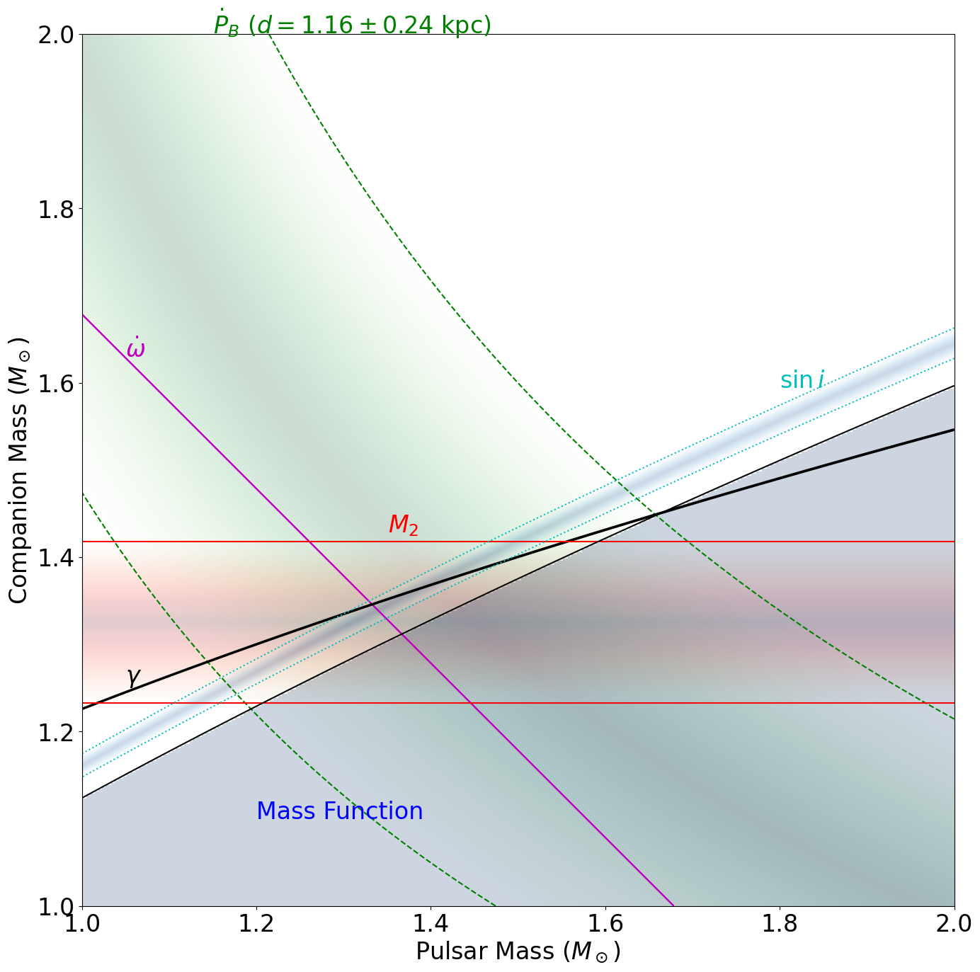
As an example we use the double neutron star (PSR B1534+12). We generate fake data, fit post-Keplerian parameters, and plot a mass-mass diagram to illustrate the overlapping constraints
This reproduces a version of Figure 9 from Fonseca et al. (2014, ApJ, 787, 82)
[1]:
from astropy import units as u, constants as c
import astropy.time
import numpy as np
from matplotlib import pyplot as plt
import matplotlib.cm as cm
import io

import pint.fitter
from pint.models import get_model
import pint.derived_quantities
import pint.simulation
import pint.logging

# setup the logging
pint.logging.setup(level="INFO")
[1]:
1
Some helper functions for plotting
[2]:
def plot_contour(mp, mc, quantity, target, uncertainty, color, nsigma=3, **kwargs):
    """Plot two lines at +/-nsigma * the uncertainty to illustrate a constraint.

    Parameters
    ----------
    mp : astropy.units.Quantity
        array of pulsar masses (x-axis)
    mc : astropy.units.Quantity
        array of companion masses (y-axis)
    quantity : astropy.units.Quantity
        2D array of the prediction as a function of mp and mc. Shape is (len(mc), len(mp))
    target : astropy.units.Quantity
        best-fit value of the prediction (say from a PINT fit).
    uncertainty : astropy.units.Quantity
        uncertainty on that best-fit
    color : str
        color string for the lines
    nsigma : float, optional
        factor times the uncertainty for the lines (default = 3)

    Returns
    -------
    `~.contour.QuadContourSet`
        See :func:`matplotlib.pyplot.contour`
    """
    return plt.contour(
        mp.value,
        mc.value,
        quantity.value,
        [(target - nsigma * uncertainty).value, (target + nsigma * uncertainty).value],
        colors=color,
        **kwargs,
    )


def plot_fill(
    mp, mc, quantity, target, uncertainty, cmap, alpha=0.2, nsigma_max=3, **kwargs
):
    """Fill a region with a color map to illustrate a constraint.

    Outside of nsigma_max * uncertainty, constraint is not shown.

    Parameters
    ----------
    mp : astropy.units.Quantity
        array of pulsar masses (x-axis)
    mc : astropy.units.Quantity
        array of companion masses (y-axis)
    quantity : astropy.units.Quantity
        2D array of the prediction as a function of mp,mc.  Shape is (len(mc),len(mp))
    target : astropy.units.Quantity
        best-fit value of the prediction (say from a PINT fit).
    uncertainty : astropy.units.Quantity
        uncertainty on that best-fit
    cmap : str or `~matplotlib.colors.Colormap`
        matplotib colormap
    alpha : float, optional
        alpha for the color fill (default = 0.2)
    nsigma_max : float, optional
        factor times the uncertainty beyond which no constraint is shown (default = 3)

    Returns
    -------
    `~matplotlib.image.AxesImage`
        See :func:`matplotlib.pyplot.imshow`
    """
    z = np.fabs((quantity - target) / uncertainty)
    z[z >= nsigma_max] = np.nan
    plt.imshow(
        z,
        origin="lower",
        extent=(mp.value.min(), mp.value.max(), mc.value.min(), mc.value.max()),
        cmap=cmap,
        alpha=alpha,
        **kwargs,
    )


def get_plot_xy(mp, mc, quantity, target, uncertainty, mp_to_plot, nsigma=3):
    """A helper function to find the point in the quantity array that is nsigma * uncertainty away
    from the target value at mp=mp_to_plot

    returns mp,mc to plot a text label

    Parameters
    ----------
    mp : astropy.units.Quantity
        array of pulsar masses (x-axis)
    mc : astropy.units.Quantity
        array of companion masses (y-axis)
    quantity : astropy.units.Quantity
        2D array of the prediction as a function of mp,mc.  Shape is (len(mc),len(mp))
    target : astropy.units.Quantity
        best-fit value of the prediction (say from a PINT fit).
    uncertainty : astropy.units.Quantity
        uncertainty on that best-fit
    mp_to_plot : astropy.units.Quantity
        x-axis value at which to interpolate
    nsigma : float, optional
        factor times the uncertainty for the lines (default = 3)

    Returns
    -------
    mp_to_plot : astropy.units.Quantity
    mc_to_plot : astropy.units.Quantity
    """
    z = (quantity - target) / uncertainty
    j = np.abs(mp - mp_to_plot).argmin()
    i = np.argmin(np.abs(z[:, j] - nsigma))
    return mp[j], mc[i]
[3]:
# par file for B1534+12 from ATNF catalog
# basically from Fonseca, Stairs, & Thorsett (2014)
# https://ui.adsabs.harvard.edu/abs/2014ApJ...787...82F/abstract
# except
# * I removed the DM1/DM2 parameters (they were causing errors without a DMEPOCH)
# * I removed RM (PINT couldn't understand it)
# * I removed EPHVER 2 (PINT doesn't do anything with it)
# * I added EPHEM DE440
test_par = """
PSRJ            J1537+1155
RAJ             15:37:09.961730               3.000e-06
DECJ            +11:55:55.43387               6.000e-05
DM              11.61944                      2.000e-05
PEPOCH          52077
F0              26.38213277689397             1.100e-13
F1              -1.686097E-15                 2.000e-21
PMRA            1.482                         7.000e-03
PMDEC           -25.285                       1.200e-02
F2              1.70E-29                      1.100e-30
BINARY          DD
PB              0.420737298879                2.000e-12
ECC             0.27367752                    7.000e-08
A1              3.7294636                     6.000e-07
T0              52076.827113263               1.100e-08
OM              283.306012                    1.200e-05
OMDOT           1.7557950                     1.900e-06
PBDOT           -0.1366E-12                   3.000e-16
#RM              10.6                          2.000e-01
PX              0.86                          1.800e-01
#DM1             -0.000653                     9.000e-06
F3              -1.6E-36                      2.000e-37
#DM2             0.00031                       1.000e-05
GAMMA           2.0708E-03                    5.000e-07
SINI            0.9772                        1.600e-03
M2              1.35                          5.000e-02
UNITS           TDB
EPHEM           DE440
"""
[4]:
# PINT wants to read from a file.  So make a file-like object
# out of the string
f = io.StringIO(test_par)
[5]:
# load the model into PINT
m = get_model(f)
[6]:
# roughly the parameters from Fonseca, Stairs, Thorsett (2014)
tstart = astropy.time.Time(1990.25, format="jyear")
tstop = astropy.time.Time(2014, format="jyear")
# this is the error on each TOA
error = 5 * u.us
# this is a guess
Ntoa = 1000
# make the new TOAs.  Note that even though `error` is passed, the TOAs
# start out perfect
tnew = pint.simulation.make_fake_toas_uniform(
    tstart.mjd * u.d, tstop.mjd * u.d, Ntoa, model=m, obs="ARECIBO", error=error
)
# So we have to still add in some noise
tnew.adjust_TOAs(astropy.time.TimeDelta(np.random.normal(size=len(tnew)) * error))
INFO     (pint.observatory              ): Applying GPS to UTC clock correction (~few nanoseconds)
INFO     (pint.observatory              ): Using global clock file for gps2utc.clk with bogus_last_correction=False
WARNING  (pint.logging                  ): /home/docs/checkouts/readthedocs.org/user_builds/nanograv-pint/envs/latest/lib/python3.11/site-packages/pint/observatory/clock_file.py:183 UserWarning: Data points out of range in clock file 'gps2utc.clk'
INFO     (pint.observatory.global_clock_corrections): File tempo/clock/time_ao.dat to be downloaded due to download policy if_missing: https://raw.githubusercontent.com/ipta/pulsar-clock-corrections/main/tempo/clock/time_ao.dat
INFO     (pint.observatory              ): Using global clock file for time_ao.dat with bogus_last_correction=False
INFO     (pint.observatory.topo_obs     ): Applying observatory clock corrections for observatory='arecibo'.
INFO     (pint.solar_system_ephemerides ): Set solar system ephemeris to de440 through astropy
INFO     (pint.models.timing_model      ): Creating a TZR TOA (AbsPhase) using the given TOAs object.
WARNING  (pint.models.absolute_phase    ): TZRMJD is not set.  Setting TZRMJD to first TOA after PEPOCH or last TOA before PEPOCH.  This may leave your residuals with an offset.
INFO     (pint.models.absolute_phase    ): The TZRSITE is set at the solar system barycenter.
INFO     (pint.models.absolute_phase    ): TZRFRQ was 0.0 or None. Setting to infinite frequency.
[7]:
# construct a PINT fitter object with the model and simulated TOAs
fit = pint.fitter.WLSFitter(tnew, m)
[8]:
# fit for all of the PK parameters
# by default because the par file doesn't have parameters listed as free
# all of the other parameters will be frozen
# so this will be an underestimate of the true uncertainties (because of covariances)
fit.model.GAMMA.frozen = False
fit.model.PBDOT.frozen = False
fit.model.OMDOT.frozen = False
fit.model.M2.frozen = False
fit.model.SINI.frozen = False
fit.fit_toas()
[8]:
np.float64(923.5839425868139)
[9]:
# look at the output.  Hopefully, since these are simulated TOAs
# the fit will be good.  And indeed we see a reduced chi^2 very close to 1
try:
    fit.print_summary()
except ValueError as e:
    print(f"Unexpected exception: {e}")
Fitted model using weighted_least_square method with 5 free parameters to 1000 TOAs
Prefit residuals Wrms = 4.810866637715858 us, Postfit residuals Wrms = 4.805163739631601 us
Chisq = 923.584 for 994 d.o.f. for reduced Chisq of 0.929

PAR                   Prefit                  Postfit            Units
============== ==================== ============================ =====
PSR                      J1537+1155 J1537+1155                   None
EPHEM                         DE440 DE440                        None
CLOCK                               TT(TAI)                      None
UNITS                           TDB TDB                          None
START                                                    47983.3 d
FINISH                                                     56658 d
BINARY                           DD DD                           None
DILATEFREQ                        N                              None
DMDATA                            N                              None
NTOA                              0                              None
CHI2                                                     923.584
CHI2R                                                   0.929159
TRES                                                     4.80516 us
POSEPOCH                      52077                              d
PX                             0.86                              mas
RAJ                 15h37m09.96173s                              hourangle
DECJ                11d55m55.43387s                              deg
PMRA                          1.482                              mas / yr
PMDEC                       -25.285                              mas / yr
F0                          26.3821                              Hz
PEPOCH                        52077                              d
F1                      -1.6861e-15                              Hz / s
F2                          1.7e-29                              Hz / s2
F3                         -1.6e-36                              Hz / s3
PLANET_SHAPIRO                    N                              None
DM                          11.6194                              pc / cm3
PB                         0.420737                              d
PBDOT                    -1.366e-13              -1.367(6)×10⁻¹³
A1                          3.72946                              lsec
A1DOT                             0                              lsec / s
ECC                        0.273678
EDOT                              0                              1 / s
T0                          52076.8                              d
OM                          283.306                              deg
OMDOT                       1.75579                 1.7557952(5) deg / yr
M2                             1.35                    1.326(31) solMass
SINI                         0.9772                   0.9799(24)
A0                                0                              s
B0                                0                              s
GAMMA                     0.0020708               0.00207058(33) s
DR                                0
DTH                               0
TZRMJD                      52081.9                              d
TZRSITE                         ssb ssb                          None
TZRFRQ                          inf                              MHz

Derived Parameters:
Period = 0.03790444117830463±0.00000000000000016 s
Pdot = (2.4224942±0.0000029)×10⁻¹⁸
Characteristic age = 2.479e+08 yr (braking index = 3)
Surface magnetic field = 9.7e+09 G
Magnetic field at light cylinder = 1639 G
Spindown Edot = 1.756e+33 erg / s (I=1e+45 cm2 g)

Binary model BinaryDD
Orbital Pdot (PBDOT) = (-1.367±0.006)×10⁻¹³ (s/s)
Total mass, assuming GR, from OMDOT is 2.6784599(12) 1 / s Msun
From SINI in model:
    cos(i) = 0.199(12)
    i = 78.5(7) deg
Pulsar mass (Shapiro Delay) = 1.315370035114187 solMass
The value of \(\dot P_B\) is biased because of kinematic effects:
Galactic acceleration
The Shklovskii effect (from the source’s proper motion) We can correct for those, following Nice & Taylor (1995, ApJ, 441, 429):
\[\dot P_{B,{\rm obs}} = \dot P_{B,{\rm true}} + P_B \left(\frac{\vec{a} \cdot \vec{n}}{c} + \frac{\mu^2 d}{c}\right)\](Eqn. 2 from that paper), where \(\vec{a} \cdot \vec{n}\) is the component of Galactic acceleration along the line of sight, \(d\) is the distance, and \(\mu\) is the proper motion. So the first term there is the Galactic acceleration term, and the second is the Shklovskii term.
For the former we need to know the Galactic potential. As a simplifying assumption we will assume a flat rotation curve, which gives us:
where
\((l,b)\) are the Galactic coordinates, \(\Theta_0\) is the rotational velocity, and \(R_0\) is the distance to the Galactic center (Eqn. 5 in the paper above).
For both of these we need to know the distance.
[10]:
# get the distance from the parallax. Note that this is crude (the inversion is not good at low S/N)
d = m.PX.quantity.to(u.kpc, equivalencies=u.parallax())
d_err = d * (m.PX.uncertainty / m.PX.quantity)
print(f"distance: {d:.2f} +/- {d_err:.2f}")
distance: 1.16 kpc +/- 0.24 kpc
[11]:
# The PBDOT measurements need correction for kinematic effects
# both Shklovskii acceleration and Galactic acceleration
# do those here

# for Galactic acceleration, need to know the size and speed of the Milky Way
# GRAVITY collaboration 2019
# https://ui.adsabs.harvard.edu/abs/2019A&A...625L..10G
R0 = 8.178 * u.kpc
Theta0 = 220 * u.km / u.s

# We will assume a flat rotation curve: not the best but probably OK
b = m.coords_as_GAL().b
l = m.coords_as_GAL().l
beta = (d / R0) * np.cos(b) - np.cos(l)
# Nice & Taylor (1995), Eqn. 5
# https://ui.adsabs.harvard.edu/abs/1995ApJ...441..429N/abstract
a_dot_n = (
    -np.cos(b) * (Theta0**2 / R0) * (np.cos(l) + beta / (np.sin(l) ** 2 + beta**2))
)
# Galactic acceleration contribution to PBDOT
PBDOT_gal = (fit.model.PB.quantity * a_dot_n / c.c).decompose()
# Shklovskii contribution
PBDOT_shk = (fit.model.PB.quantity * pint.utils.pmtot(m) ** 2 * d / c.c).to(
    u.s / u.s, equivalencies=u.dimensionless_angles()
)
# the uncertainty from the Galactic acceleration isn't included
# but it's much smaller than the Shklovskii term so we'll ignore it
PBDOT_err = (fit.model.PB.quantity * pint.utils.pmtot(m) ** 2 * d_err / c.c).to(
    u.s / u.s, equivalencies=u.dimensionless_angles()
)
print(f"PBDOT_gal = {PBDOT_gal:.2e}, PBDOT_shk = {PBDOT_shk:.2e} +/- {PBDOT_err:.2e}")
PBDOT_gal = 1.20e-15, PBDOT_shk = 6.59e-14 +/- 1.38e-14
[12]:
# make a dense grid of Mp,Mc values to compute all of the PK parameters
mp = np.linspace(1, 2, 500) * u.Msun
mc = np.linspace(1, 2, 400) * u.Msun
Mp, Mc = np.meshgrid(mp, mc)
omdot_pred = pint.derived_quantities.omdot(
    Mp, Mc, fit.model.PB.quantity, fit.model.ECC.quantity
)
pbdot_pred = pint.derived_quantities.pbdot(
    Mp, Mc, fit.model.PB.quantity, fit.model.ECC.quantity
)
gamma_pred = pint.derived_quantities.gamma(
    Mp, Mc, fit.model.PB.quantity, fit.model.ECC.quantity
)
sini_pred = (
    pint.derived_quantities.mass_funct(fit.model.PB.quantity, fit.model.A1.quantity)
    * (Mp + Mc) ** 2
    / Mc**3
) ** (1.0 / 3)

plt.figure(figsize=(16, 16))
fontsize = 24

nsigma = 3

# OMDOT
# for each quantity we plot contours at +/-3 sigma compared to the best fit
# we also (optionally) plot a colored fill if there is enough space
# and then try to label it
# (a little fudging is required for that)
plot_contour(
    mp, mc, omdot_pred, fit.model.OMDOT.quantity, fit.model.OMDOT.uncertainty, "m"
)
# this one doesn't have enough space to really display
# plot_fill(mp, mc, omdot_pred, fit.model.OMDOT.quantity,fit.model.OMDOT.uncertainty, cmap=cm.Reds_r)
x, y = get_plot_xy(
    mp,
    mc,
    omdot_pred,
    fit.model.OMDOT.quantity,
    fit.model.OMDOT.uncertainty,
    1.05 * u.Msun,
    3,
)
plt.text(x.value, y.value, "$\dot \omega$", fontsize=fontsize, color="m")

# PBDOT
# make sure we correct it for the kinematic terms
PBDOT_corr = fit.model.PBDOT.quantity - PBDOT_gal - PBDOT_shk
# also add the error from the distance uncertainty in quadrature
PBDOT_uncertainty = np.sqrt(fit.model.PBDOT.uncertainty**2 + PBDOT_err**2)
plot_contour(mp, mc, pbdot_pred, PBDOT_corr, PBDOT_uncertainty, "g", linestyles="--")
plot_fill(mp, mc, pbdot_pred, PBDOT_corr, PBDOT_uncertainty, cmap=cm.Greens_r)
x, y = get_plot_xy(mp, mc, pbdot_pred, PBDOT_corr, PBDOT_uncertainty, 1.15 * u.Msun, -3)
plt.text(
    x.value,
    y.value,
    "$\dot P_B$ ($d=%.2f \pm %.2f$ kpc)" % (d.value, d_err.value),
    fontsize=fontsize,
    color="g",
)

# GAMMA
plot_contour(
    mp, mc, gamma_pred, fit.model.GAMMA.quantity, fit.model.GAMMA.uncertainty, "k"
)
# plot_fill(mp, mc, gamma_pred, fit.model.GAMMA.quantity,fit.model.GAMMA.uncertainty, cmap=cm.Greens_r)
x, y = get_plot_xy(
    mp,
    mc,
    gamma_pred,
    fit.model.GAMMA.quantity,
    fit.model.GAMMA.uncertainty,
    1.05 * u.Msun,
    3,
)
plt.text(x.value, y.value + 0.01, "$\gamma$", fontsize=fontsize, color="k")

# M2
plot_contour(mp, mc, Mc, fit.model.M2.quantity, fit.model.M2.uncertainty, "r")
plot_fill(mp, mc, Mc, fit.model.M2.quantity, fit.model.M2.uncertainty, cmap=cm.Reds_r)
x, y = get_plot_xy(
    mp, mc, Mc, fit.model.M2.quantity, fit.model.M2.uncertainty, 1.35 * u.Msun, 3
)
plt.text(x.value, y.value + 0.01, "$M_2$", fontsize=fontsize, color="r")

# SINI
plot_contour(
    mp,
    mc,
    sini_pred,
    fit.model.SINI.quantity,
    fit.model.SINI.uncertainty,
    "c",
    linestyles=":",
)
plot_fill(
    mp,
    mc,
    sini_pred,
    fit.model.SINI.quantity,
    fit.model.SINI.uncertainty,
    cmap=cm.Blues_r,
)
x, y = get_plot_xy(
    mp,
    mc,
    sini_pred,
    fit.model.SINI.quantity,
    fit.model.SINI.uncertainty,
    1.8 * u.Msun,
    -3,
)
plt.text(x.value, y.value + 0.02, "$\sin i$", fontsize=fontsize, color="c")

# Mass function
plt.contour(
    mp.value,
    mc.value,
    pint.derived_quantities.mass_funct2(Mp, Mc, 90 * u.deg).value,
    [
        pint.derived_quantities.mass_funct(
            fit.model.PB.quantity, fit.model.A1.quantity
        ).value
    ],
    colors="k",
)
z = (
    pint.derived_quantities.mass_funct2(Mp, Mc, 90 * u.deg).value
    - pint.derived_quantities.mass_funct(
        fit.model.PB.quantity, fit.model.A1.quantity
    ).value
)
z[z > 0] = np.nan
z[z <= 0] = 1
plt.imshow(
    z,
    origin="lower",
    extent=(mp.value.min(), mp.value.max(), mc.value.min(), mc.value.max()),
    cmap=cm.Blues,
    vmin=0,
    vmax=1,
    alpha=0.2,
)
# plt.contour(mp.value,mc.value,gamma_pred.value,[(f.model.GAMMA.quantity - 3*f.model.GAMMA.uncertainty).value,(f.model.GAMMA.quantity + 3*f.model.GAMMA.uncertainty).value])
# plt.contour(mp.value,mc.value,pbdot_pred.value,[(f.model.PBDOT.quantity - 3*f.model.PBDOT.uncertainty).value,(f.model.PBDOT.quantity + 3*f.model.PBDOT.uncertainty).value])
plt.text(1.2, 1.1, "Mass Function", fontsize=fontsize, color="b")

plt.xlabel("Pulsar Mass $(M_\\odot)$", fontsize=fontsize)
plt.ylabel("Companion Mass $(M_\\odot)$", fontsize=fontsize)
plt.xticks(fontsize=fontsize)
plt.yticks(fontsize=fontsize)
# plt.savefig('PSRB1534_massmass.png')
[12]:
(array([1. , 1.2, 1.4, 1.6, 1.8, 2. ]),
 [Text(0, 1.0, '1.0'),
  Text(0, 1.2000000000000002, '1.2'),
  Text(0, 1.4000000000000001, '1.4'),
  Text(0, 1.6, '1.6'),
  Text(0, 1.8, '1.8'),
  Text(0, 2.0, '2.0')])
[ ]: