This Jupyter notebook can be downloaded from Wideband_TOA_walkthrough.ipynb, or viewed as a python script at Wideband_TOA_walkthrough.py.
Wideband TOA fitting
Traditional pulsar timing involved measuring only the arrival time of each pulse. But as receivers have covered wider and wider contiguous bandwidths, it became necessary to generate many TOAs for each time interval, covering different subbands. This frequency coverage allowed better handling of changing dispersion measures, but resulted in a large number of TOAs and had certain limitations. A new approach measures the pulse arrival time and the dispersion measure simultaneously from a frequency-resolved data cube. This produces TOAs, each of which has an associated dispersion measure and uncertainty. Working with this data requires different handling from PINT. This notebook demonstrates that.
[1]:
import astropy.units as u
import matplotlib.pyplot as plt
from astropy.visualization import quantity_support

from pint.fitter import Fitter
from pint.models import get_model_and_toas
import pint.config
import pint.logging

# setup logging
pint.logging.setup(level="INFO")

quantity_support()
[1]:
<astropy.visualization.units.quantity_support.<locals>.MplQuantityConverterFormatted at 0x740cf4df5110>
Set up your inputs
[2]:
model, toas = get_model_and_toas(
    pint.config.examplefile("J1614-2230_NANOGrav_12yv3.wb.gls.par"),
    pint.config.examplefile("J1614-2230_NANOGrav_12yv3.wb.tim"),
)
INFO     (pint.models.parameter         ): Parameter PBDOT's value will be scaled by 1e-12
INFO     (pint.models.parameter         ): Parameter PBDOT's value will be scaled by 1e-12
INFO     (pint.observatory              ): Applying GPS to UTC clock correction (~few nanoseconds)
INFO     (pint.observatory              ): Using global clock file for gps2utc.clk with bogus_last_correction=False
INFO     (pint.observatory              ): Applying TT(TAI) to TT(BIPM2017) clock correction (~27 us)
INFO     (pint.observatory              ): Loading BIPM clock version bipm2017
INFO     (pint.observatory.global_clock_corrections): File T2runtime/clock/tai2tt_bipm2017.clk to be downloaded due to download policy if_missing: https://raw.githubusercontent.com/ipta/pulsar-clock-corrections/main/T2runtime/clock/tai2tt_bipm2017.clk
INFO     (pint.observatory              ): Using global clock file for tai2tt_bipm2017.clk with bogus_last_correction=True
INFO     (pint.observatory.clock_file   ): Disregarding suspicious MJD -2612.5 in TEMPO clock file
INFO     (pint.observatory              ): Using global clock file for time_gbt.dat with bogus_last_correction=False
INFO     (pint.observatory.topo_obs     ): Applying observatory clock corrections for observatory='gbt'.
INFO     (pint.solar_system_ephemerides ): Set solar system ephemeris to de436 from download
The DM and its uncertainty are recorded as flags, pp_dm and pp_dme on the TOAs that have them, They are not currently available as Columns in the Astropy object. On the other hand, it is not necessary that every observation have a measured DM.
(The name, pp_dm, refers to the fact that they are obtained using “phase portraits”, like profiles but in one more dimension.)
[3]:
print(open(toas.filename).readlines()[-1])
guppi_57922_J1614-2230_0006.12y.x.ff 812.60505020 57922.064007172196642 0.419 gbt -pp_dm 34.4877666 -pp_dme 0.0004867 -be GUPPI -ver 20200204 -nchx 55 -tobs 891.204 -f Rcvr_800_GUPPI -gof 1.041 -snr 169.071 -fratio 1.258 -pta NANOGrav -subint 1 -nch 64 -flux 2.43148 -bw 187.435 -chbw 3.125 -fe Rcvr_800 -fluxe 0.01498 -nbin 2048 -proc 12y -tmplt J1614-2230.Rcvr_800.GUPPI.12y.x.avg_port.spl -flux_ref_freq 836.73551
[4]:
toas.table[-1]
[4]:
| index | mjd | mjd_float | error | freq | obs | flags | delta_pulse_number | tdb | tdbld | ssb_obs_pos | ssb_obs_vel | obs_sun_pos |
|---|---|---|---|---|---|---|---|---|---|---|---|---|
| d | us | MHz | km | km / s | km | |||||||
| int64 | object | float64 | float64 | float64 | str3 | object | float64 | object | float128 | float64[3] | float64[3] | float64[3] |
| 274 | 57922.06400717255 | 57922.06400717254 | 0.419 | 812.6050502 | gbt | {'format': 'Tempo2', 'name': 'guppi_57922_J1614-2230_0006.12y.x.ff', 'pp_dm': '34.4877666', 'pp_dme': '0.0004867', 'be': 'GUPPI', 'ver': '20200204', 'nchx': '55', 'tobs': '891.204', 'f': 'Rcvr_800_GUPPI', 'gof': '1.041', 'snr': '169.071', 'fratio': '1.258', 'pta': 'NANOGrav', 'subint': '1', 'nch': '64', 'flux': '2.43148', 'bw': '187.435', 'chbw': '3.125', 'fe': 'Rcvr_800', 'fluxe': '0.01498', 'nbin': '2048', 'proc': '12y', 'tmplt': 'J1614-2230.Rcvr_800.GUPPI.12y.x.avg_port.spl', 'flux_ref_freq': '836.73551', 'clkcorr': '3.023951845889943e-05'} | 0.0 | 57922.06480791843 | 57922.064807918432745 | -8106233.828294313 .. -60075124.09656769 | 29.431081448790245 .. -0.7083729035832717 | 8524988.622096533 .. 60354832.968297414 |
[5]:
toas.table["flags"][0]
[5]:
FlagDict({'format': 'Tempo2', 'name': '54724.000006.1.000.000.9y.x.ff', 'pp_dm': '34.4828090', 'pp_dme': '0.0118764', 'be': 'GASP', 'ver': '20200204', 'nchx': '16', 'tobs': '60.078', 'f': 'Rcvr_800_GASP', 'gof': '1.035', 'snr': '35.572', 'fratio': '1.073', 'pta': 'NANOGrav', 'subint': '0', 'nch': '16', 'bw': '60.000', 'chbw': '4.000', 'fe': 'Rcvr_800', 'nbin': '2048', 'proc': '12y', 'tmplt': 'J1614-2230.Rcvr_800.GUPPI.12y.x.avg_port.spl', 'to': '-8.970e-07', 'clkcorr': '2.6166525221999545e-05'})
Do the fit
As before, but now we need a fitter adapted to wideband TOAs. The function Fitter.auto() will examine the model and choose an appropriate one.
[6]:
fitter = Fitter.auto(toas, model)
INFO     (pint.fitter                   ): For wideband TOAs and downhill fitter, returning 'WidebandDownhillFitter'
INFO     (pint.observatory              ): Applying TT(TAI) to TT(BIPM2023) clock correction (~27 us)
INFO     (pint.observatory              ): Loading BIPM clock version bipm2023
INFO     (pint.observatory              ): Using global clock file for tai2tt_bipm2023.clk with bogus_last_correction=False
[7]:
fitter.fit_toas()
WARNING  (pint.logging                  ): /home/docs/checkouts/readthedocs.org/user_builds/nanograv-pint/envs/latest/lib/python3.11/site-packages/pint/fitter.py:2046 UserWarning: The current version of WidebandTOAFitter does not support models with correlated errors.
WARNING  (pint.logging                  ): /home/docs/checkouts/readthedocs.org/user_builds/nanograv-pint/envs/latest/lib/python3.11/site-packages/pint/fitter.py:2046 UserWarning: The current version of WidebandTOAFitter does not support models with correlated errors.
WARNING  (pint.logging                  ): /home/docs/checkouts/readthedocs.org/user_builds/nanograv-pint/envs/latest/lib/python3.11/site-packages/pint/fitter.py:2046 UserWarning: The current version of WidebandTOAFitter does not support models with correlated errors.
[7]:
True
What is new, compared to narrowband fitting?
Residual objects combine TOA and time data
[8]:
type(fitter.resids)
[8]:
pint.residuals.WidebandTOAResiduals
If we look into the resids attribute, it has two independent Residual objects.
[9]:
fitter.resids.toa, fitter.resids.dm
[9]:
(<pint.residuals.Residuals at 0x740cf1dded10>,
 <pint.residuals.WidebandDMResiduals at 0x740ce4b59190>)
Each of them can be used independently
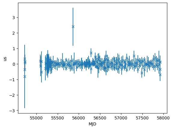
Time residual
[10]:
time_resids = fitter.resids.toa.time_resids
plt.errorbar(
    toas.get_mjds().value,
    time_resids.to_value(u.us),
    yerr=toas.get_errors().to_value(u.us),
    fmt="x",
)
plt.ylabel("us")
plt.xlabel("MJD")
[10]:
Text(0.5, 0, 'MJD')
[11]:
# Time RMS
print(fitter.resids.toa.rms_weighted())
print(fitter.resids.toa.chi2)
0.17493097727770984 us
156.75062456725067
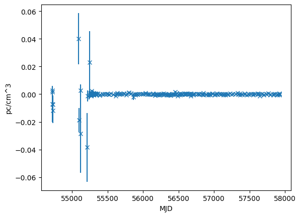
DM residual
[12]:
dm_resids = fitter.resids.dm.resids
dm_error = fitter.resids.dm.get_data_error()
plt.errorbar(toas.get_mjds().value, dm_resids.value, yerr=dm_error.value, fmt="x")
plt.ylabel("pc/cm^3")
plt.xlabel("MJD")
[12]:
Text(0.5, 0, 'MJD')
[13]:
# DM RMS
print(fitter.resids.dm.rms_weighted())
print(fitter.resids.dm.chi2)
0.00035817066441693124 pc / cm3
276.4200665058503
However, in the combined residuals, one can access rms and chi2 as well
[14]:
print(fitter.resids.rms_weighted())
print(fitter.resids.chi2)
{'toa': <Quantity 1.74930977e-07 s>, 'dm': <Quantity 0.00035817 pc / cm3>}
433.17069107310084
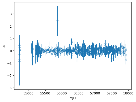
The initial residuals is also a combined residual object
[15]:
time_resids = fitter.resids_init.toa.time_resids
plt.errorbar(
    toas.get_mjds().value,
    time_resids.to_value(u.us),
    yerr=toas.get_errors().to_value(u.us),
    fmt="x",
)
plt.ylabel("us")
plt.xlabel("MJD")
[15]:
Text(0.5, 0, 'MJD')
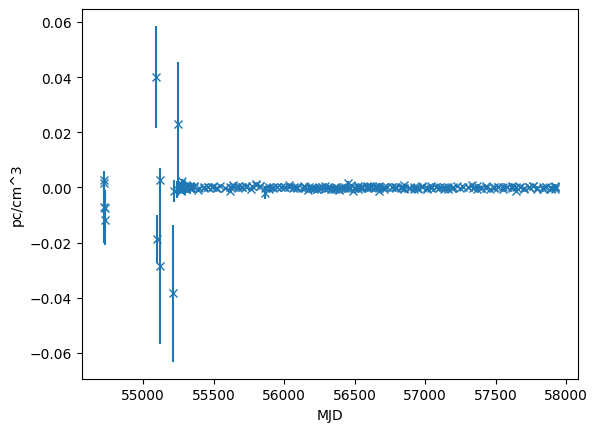
[16]:
dm_resids = fitter.resids_init.dm.resids
dm_error = fitter.resids_init.dm.get_data_error()
plt.errorbar(toas.get_mjds().value, dm_resids.value, yerr=dm_error.value, fmt="x")
plt.ylabel("pc/cm^3")
plt.xlabel("MJD")
[16]:
Text(0.5, 0, 'MJD')
Matrices
We’re now fitting a mixed set of data, so the matrices used in fitting now have different units in different parts, and some care is needed to keep track of which part goes where.
Design Matrix are combined
[17]:
d_matrix, labels, units = fitter.get_designmatrix()
[18]:
print("Number of TOAs:", toas.ntoas)
print("Number of DM measurments:", len(fitter.resids.dm.dm_data))
print("Number of fit params:", len(fitter.model.free_params))
print("Shape of design matrix:", d_matrix.shape)
Number of TOAs: 275
Number of DM measurments: 275
Number of fit params: 130
Shape of design matrix: (275, 131)
Covariance Matrix are combined
[19]:
# c_matrix = fitter.get_noise_covariancematrix()
[20]:
# print("Shape of covariance matrix:", c_matrix.shape)
NOTE the matrix are PINTMatrix object right now, here are the difference
If you want to access the matrix data
[21]:
# print(d_matrix.matrix)
PINT matrix has labels that marks all the element in the matrix. It has the label name, index of range of the matrix, and the unit.
[22]:
# print("labels for dimension 0:", d_matrix.labels[0])
[ ]: